

Analog.Examples.ChuaCircuit
Chua's circuit, an electronic circuit known for its chaotic dynamics.
This component represents Chua's circuit, a relatively simple electronic system capable of exhibiting complex nonlinear dynamics, including bifurcations and chaos. The circuit is constructed from two capacitors (capacitor1, capacitor2), one inductor (inductor), a linear resistor (resistor), a linear conductor (conductor), and a single nonlinear element known as Chua's diode (represented by nonlinear_resistor). The behavior of the circuit is typically described by a set of three first-order autonomous ordinary differential equations for the voltage across each capacitor and the current through the inductor.
The current i_NR through the nonlinear_resistor as a function of the voltage v_C1 across it is given by:
The governing differential equations for the circuit are (using v_C1 for capacitor1.v, v_C2 for capacitor2.v, i_L for inductor.i):
Initial conditions for capacitor1.v, capacitor2.v, and inductor.i are specified within the relations block to define the starting state of the simulation.
Usage
ElectricalComponents.Analog.Examples.ChuaCircuit()
Behavior
Source
"""
Chua's circuit, an electronic circuit known for its chaotic dynamics.

This component represents Chua's circuit, a relatively simple electronic system
capable of exhibiting complex nonlinear dynamics, including bifurcations and
chaos. The circuit is constructed from two capacitors (`capacitor1`, `capacitor2`),
one inductor (`inductor`), a linear resistor (`resistor`), a linear conductor
(`conductor`), and a single nonlinear element known as Chua's diode (represented
by `nonlinear_resistor`). The behavior of the circuit is typically described by a
set of three first-order autonomous ordinary differential equations for the
voltage across each capacitor and the current through the inductor.

The current `i_NR` through the `nonlinear_resistor` as a function of the voltage `v_C1` across it is given by:
```math
i_{NR}(v_{C1}) = Gb \cdot v_{C1} + \frac{1}{2}(Ga - Gb)(|v_{C1} + Ve| - |v_{C1} - Ve|)
```
The governing differential equations for the circuit are (using `v_C1` for `capacitor1.v`, `v_C2` for `capacitor2.v`, `i_L` for `inductor.i`):
```math
capacitor1.C \cdot \frac{d(v_{C1})}{dt} = conductor.G \cdot (v_{C2} - v_{C1}) - i_{NR}(v_{C1})
```
```math
capacitor2.C \cdot \frac{d(v_{C2})}{dt} = conductor.G \cdot (v_{C1} - v_{C2}) - i_L
```
```math
inductor.L \cdot \frac{d(i_L)}{dt} = v_{C2} - resistor.R \cdot i_L
```
Initial conditions for `capacitor1.v`, `capacitor2.v`, and `inductor.i` are
specified within the `relations` block to define the starting state of the simulation.
"""
example component ChuaCircuit
  "Inductor of the Chua's circuit."
  inductor = ElectricalComponents.Analog.Basic.Inductor(L = 18) {
    "Dyad": {
      "placement": {
        "icon": {"iconName": "default", "x1": 0, "y1": 100, "x2": 100, "y2": 200, "rot": 90},
        "diagram": {"iconName": "default", "x1": 60, "y1": 120, "x2": 160, "y2": 220, "rot": 90}
      },
      "tags": []
    }
  }
  "Linear resistor, typically in series with the inductor."
  resistor = ElectricalComponents.Analog.Basic.Resistor(R = 12.5e-3) {
    "Dyad": {
      "placement": {
        "icon": {"iconName": "default", "x1": 0, "y1": 250, "x2": 100, "y2": 350, "rot": 90},
        "diagram": {"iconName": "default", "x1": 60, "y1": 300, "x2": 160, "y2": 400, "rot": 90}
      },
      "tags": []
    }
  }
  "Linear conductor, connecting the two capacitors."
  conductor = ElectricalComponents.Analog.Basic.Conductor(G = 0.565) {
    "Dyad": {
      "placement": {
        "icon": {"iconName": "default", "x1": 225, "y1": 25, "x2": 325, "y2": 125, "rot": 0},
        "diagram": {"iconName": "default", "x1": 460, "y1": 20, "x2": 560, "y2": 120, "rot": 0}
      },
      "tags": []
    }
  }
  "First capacitor in the Chua's circuit."
  capacitor1 = ElectricalComponents.Analog.Basic.Capacitor(C = 10) {
    "Dyad": {
      "placement": {
        "icon": {"iconName": "default", "x1": 300, "y1": 175, "x2": 400, "y2": 275, "rot": 90},
        "diagram": {"iconName": "default", "x1": 700, "y1": 180, "x2": 800, "y2": 280, "rot": 90}
      },
      "tags": []
    }
  }
  "Second capacitor in the Chua's circuit."
  capacitor2 = ElectricalComponents.Analog.Basic.Capacitor(C = 100) {
    "Dyad": {
      "placement": {
        "icon": {"iconName": "default", "x1": 150, "y1": 175, "x2": 250, "y2": 275, "rot": 90},
        "diagram": {"iconName": "default", "x1": 270, "y1": 190, "x2": 370, "y2": 290, "rot": 90}
      },
      "tags": []
    }
  }
  "Nonlinear resistor representing the Chua's diode, with parameters Ga, Gb, Ve."
  nonlinear_resistor = ElectricalComponents.Analog.Basic.NonlinearResistor(Ga = -0.757576, Gb = -0.409091, Ve = 1) {
    "Dyad": {
      "placement": {
        "icon": {"iconName": "default", "x1": 450, "y1": 175, "x2": 550, "y2": 275, "rot": 90},
        "diagram": {"iconName": "default", "x1": 880, "y1": 180, "x2": 980, "y2": 280, "rot": 90}
      },
      "tags": []
    }
  }
  "Ground reference for the circuit."
  ground = ElectricalComponents.Analog.Basic.Ground() {
    "Dyad": {
      "placement": {
        "icon": {"iconName": "default", "x1": 225, "y1": 400, "x2": 325, "y2": 500, "rot": 0},
        "diagram": {"iconName": "default", "x1": 450, "y1": 500, "x2": 550, "y2": 600, "rot": 0}
      },
      "tags": []
    }
  }
relations
  initial inductor.i = 0
  initial capacitor1.v = 4
  initial capacitor2.v = 0
  connect(inductor.n, resistor.p) {"Dyad": {"edges": [{"S": 1, "M": [], "E": 2}], "renderStyle": "standard"}}
  connect(conductor.p, inductor.p) {
    "Dyad": {
      "edges": [{"S": 1, "M": [{"x": 110, "y": 70}], "E": 2}],
      "renderStyle": "standard"
    }
  }
  connect(nonlinear_resistor.p, conductor.n) {
    "Dyad": {
      "edges": [{"S": 1, "M": [{"x": 930, "y": 70}], "E": 2}],
      "renderStyle": "standard"
    }
  }
  connect(capacitor2.n, resistor.n) {
    "Dyad": {
      "edges": [{"S": 1, "M": [{"x": 320, "y": 460}, {"x": 110, "y": 460}], "E": 2}],
      "renderStyle": "standard"
    }
  }
  connect(capacitor1.p, conductor.n) {
    "Dyad": {
      "edges": [{"S": 1, "M": [{"x": 750, "y": 70}], "E": 2}],
      "renderStyle": "standard"
    }
  }
  connect(inductor.p, capacitor2.p) {
    "Dyad": {
      "edges": [{"S": 1, "M": [{"x": 110, "y": 70}, {"x": 320, "y": 70}], "E": 2}],
      "renderStyle": "standard"
    }
  }
  connect(ground.g, resistor.n) {
    "Dyad": {
      "edges": [{"S": 1, "M": [{"x": 500, "y": 460}, {"x": 110, "y": 460}], "E": 2}],
      "renderStyle": "standard"
    }
  }
  connect(capacitor1.n, ground.g) {
    "Dyad": {
      "edges": [{"S": 1, "M": [{"x": 750, "y": 460}, {"x": 500, "y": 460}], "E": 2}],
      "renderStyle": "standard"
    }
  }
  connect(nonlinear_resistor.n, ground.g) {
    "Dyad": {
      "edges": [{"S": 1, "M": [{"x": 930, "y": 460}, {"x": 500, "y": 460}], "E": 2}],
      "renderStyle": "standard"
    }
  }
metadata {
  "Dyad": {
    "icons": {"default": "dyad://ElectricalComponents/Example.svg"},
    "tests": {
      "case1": {
        "stop": 200,
        "reltol": 1e-9,
        "abstol": 1e-9,
        "expect": {"signals": ["capacitor1.v"]}
      }
    }
  }
}
end
Flattened Source
"""
Chua's circuit, an electronic circuit known for its chaotic dynamics.

This component represents Chua's circuit, a relatively simple electronic system
capable of exhibiting complex nonlinear dynamics, including bifurcations and
chaos. The circuit is constructed from two capacitors (`capacitor1`, `capacitor2`),
one inductor (`inductor`), a linear resistor (`resistor`), a linear conductor
(`conductor`), and a single nonlinear element known as Chua's diode (represented
by `nonlinear_resistor`). The behavior of the circuit is typically described by a
set of three first-order autonomous ordinary differential equations for the
voltage across each capacitor and the current through the inductor.

The current `i_NR` through the `nonlinear_resistor` as a function of the voltage `v_C1` across it is given by:
```math
i_{NR}(v_{C1}) = Gb \cdot v_{C1} + \frac{1}{2}(Ga - Gb)(|v_{C1} + Ve| - |v_{C1} - Ve|)
```
The governing differential equations for the circuit are (using `v_C1` for `capacitor1.v`, `v_C2` for `capacitor2.v`, `i_L` for `inductor.i`):
```math
capacitor1.C \cdot \frac{d(v_{C1})}{dt} = conductor.G \cdot (v_{C2} - v_{C1}) - i_{NR}(v_{C1})
```
```math
capacitor2.C \cdot \frac{d(v_{C2})}{dt} = conductor.G \cdot (v_{C1} - v_{C2}) - i_L
```
```math
inductor.L \cdot \frac{d(i_L)}{dt} = v_{C2} - resistor.R \cdot i_L
```
Initial conditions for `capacitor1.v`, `capacitor2.v`, and `inductor.i` are
specified within the `relations` block to define the starting state of the simulation.
"""
example component ChuaCircuit
  "Inductor of the Chua's circuit."
  inductor = ElectricalComponents.Analog.Basic.Inductor(L = 18) {
    "Dyad": {
      "placement": {
        "icon": {"iconName": "default", "x1": 0, "y1": 100, "x2": 100, "y2": 200, "rot": 90},
        "diagram": {"iconName": "default", "x1": 60, "y1": 120, "x2": 160, "y2": 220, "rot": 90}
      },
      "tags": []
    }
  }
  "Linear resistor, typically in series with the inductor."
  resistor = ElectricalComponents.Analog.Basic.Resistor(R = 12.5e-3) {
    "Dyad": {
      "placement": {
        "icon": {"iconName": "default", "x1": 0, "y1": 250, "x2": 100, "y2": 350, "rot": 90},
        "diagram": {"iconName": "default", "x1": 60, "y1": 300, "x2": 160, "y2": 400, "rot": 90}
      },
      "tags": []
    }
  }
  "Linear conductor, connecting the two capacitors."
  conductor = ElectricalComponents.Analog.Basic.Conductor(G = 0.565) {
    "Dyad": {
      "placement": {
        "icon": {"iconName": "default", "x1": 225, "y1": 25, "x2": 325, "y2": 125, "rot": 0},
        "diagram": {"iconName": "default", "x1": 460, "y1": 20, "x2": 560, "y2": 120, "rot": 0}
      },
      "tags": []
    }
  }
  "First capacitor in the Chua's circuit."
  capacitor1 = ElectricalComponents.Analog.Basic.Capacitor(C = 10) {
    "Dyad": {
      "placement": {
        "icon": {"iconName": "default", "x1": 300, "y1": 175, "x2": 400, "y2": 275, "rot": 90},
        "diagram": {"iconName": "default", "x1": 700, "y1": 180, "x2": 800, "y2": 280, "rot": 90}
      },
      "tags": []
    }
  }
  "Second capacitor in the Chua's circuit."
  capacitor2 = ElectricalComponents.Analog.Basic.Capacitor(C = 100) {
    "Dyad": {
      "placement": {
        "icon": {"iconName": "default", "x1": 150, "y1": 175, "x2": 250, "y2": 275, "rot": 90},
        "diagram": {"iconName": "default", "x1": 270, "y1": 190, "x2": 370, "y2": 290, "rot": 90}
      },
      "tags": []
    }
  }
  "Nonlinear resistor representing the Chua's diode, with parameters Ga, Gb, Ve."
  nonlinear_resistor = ElectricalComponents.Analog.Basic.NonlinearResistor(Ga = -0.757576, Gb = -0.409091, Ve = 1) {
    "Dyad": {
      "placement": {
        "icon": {"iconName": "default", "x1": 450, "y1": 175, "x2": 550, "y2": 275, "rot": 90},
        "diagram": {"iconName": "default", "x1": 880, "y1": 180, "x2": 980, "y2": 280, "rot": 90}
      },
      "tags": []
    }
  }
  "Ground reference for the circuit."
  ground = ElectricalComponents.Analog.Basic.Ground() {
    "Dyad": {
      "placement": {
        "icon": {"iconName": "default", "x1": 225, "y1": 400, "x2": 325, "y2": 500, "rot": 0},
        "diagram": {"iconName": "default", "x1": 450, "y1": 500, "x2": 550, "y2": 600, "rot": 0}
      },
      "tags": []
    }
  }
relations
  initial inductor.i = 0
  initial capacitor1.v = 4
  initial capacitor2.v = 0
  connect(inductor.n, resistor.p) {"Dyad": {"edges": [{"S": 1, "M": [], "E": 2}], "renderStyle": "standard"}}
  connect(conductor.p, inductor.p) {
    "Dyad": {
      "edges": [{"S": 1, "M": [{"x": 110, "y": 70}], "E": 2}],
      "renderStyle": "standard"
    }
  }
  connect(nonlinear_resistor.p, conductor.n) {
    "Dyad": {
      "edges": [{"S": 1, "M": [{"x": 930, "y": 70}], "E": 2}],
      "renderStyle": "standard"
    }
  }
  connect(capacitor2.n, resistor.n) {
    "Dyad": {
      "edges": [{"S": 1, "M": [{"x": 320, "y": 460}, {"x": 110, "y": 460}], "E": 2}],
      "renderStyle": "standard"
    }
  }
  connect(capacitor1.p, conductor.n) {
    "Dyad": {
      "edges": [{"S": 1, "M": [{"x": 750, "y": 70}], "E": 2}],
      "renderStyle": "standard"
    }
  }
  connect(inductor.p, capacitor2.p) {
    "Dyad": {
      "edges": [{"S": 1, "M": [{"x": 110, "y": 70}, {"x": 320, "y": 70}], "E": 2}],
      "renderStyle": "standard"
    }
  }
  connect(ground.g, resistor.n) {
    "Dyad": {
      "edges": [{"S": 1, "M": [{"x": 500, "y": 460}, {"x": 110, "y": 460}], "E": 2}],
      "renderStyle": "standard"
    }
  }
  connect(capacitor1.n, ground.g) {
    "Dyad": {
      "edges": [{"S": 1, "M": [{"x": 750, "y": 460}, {"x": 500, "y": 460}], "E": 2}],
      "renderStyle": "standard"
    }
  }
  connect(nonlinear_resistor.n, ground.g) {
    "Dyad": {
      "edges": [{"S": 1, "M": [{"x": 930, "y": 460}, {"x": 500, "y": 460}], "E": 2}],
      "renderStyle": "standard"
    }
  }
metadata {
  "Dyad": {
    "icons": {"default": "dyad://ElectricalComponents/Example.svg"},
    "tests": {
      "case1": {
        "stop": 200,
        "reltol": 1e-9,
        "abstol": 1e-9,
        "expect": {"signals": ["capacitor1.v"]}
      }
    }
  }
}
end
Test Cases
Test Case case1
plt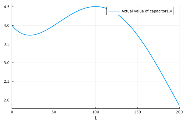
Related
Examples
Experiments
Analyses