TUTORIAL

Design Optimization

In this demo we will show how to:

• build a model from scratch using Dyad and standard library components

• perform a design optimization using DyadModelOptimizer.jl to satisfy a given design specification.

In this example, we will design a stopper for a runaway train. We assume the following design specification:

1. The stopper needs to stop the train within 2 meters.

2. The stopper needs to do so at an acceleration less than 5*g.

By the end, we should have something that looks like this:

To get started, we shall launch the Dyad Studio application on JuliaHub. When the app finishes launching, you will land in a VS Code environment. Run the "Dyad: Create Library" command in the command palette (shift + control + p), and create a new library named "DyadTutorial".

Building the System

We will design a stopper for a runaway train. The train is modeled as a series of connected train cars, and the stopper is modeled as a simple damped spring.

We can use standard components from the TranslationalComponents library.

using Pkg
Pkg.add(["TranslationalComponents"])

We will then create a feedback control system as given below:

Train Cars

First, let's design the train cars. This should be written to a file named dyad/train_cars.dyad.

We model each train car as a mass, coupled via a spring damper on each side to another train car. The mass is modeled as a system with two flanges, mechanical connection points that transmit force.

Solving the System

# using <LibraryName>
using DyadInterface
res = TrainCarsTransientAnalysis()

Transient Analysis Solution for traincar.TrainCars
with 8 differential equations and 0 algebraic equations

retcode: Success
Interpolation: 3rd order Hermite
t: 22-element Vector{Float64}: [0.0, 0.020011592337321558 … 0.9485546765314725, 1.0]
u: 22-element Vector{Vector{Float64}}:
 [3.45, 2.45, 10.0, 1.45, 10.0, 0.45, 10.0, 10.0]
 [3.65012, 2.65012, 10.0, 1.65012, 10.0, 0.650116, 10.0, 10.0]
 [5.58865, 4.58865, 10.0, 3.58865, 10.0, 2.58865, 10.0, 10.0]
 [5.7632, 4.7632, 10.0, 3.7632, 9.99998, 2.7632, 9.99999, 10.0]
 [5.86505, 4.86505, 10.0, 3.86505, 9.99998, 2.86505, 9.99999, 10.0]
 [5.95903, 4.95903, 10.0, 3.95903, 9.99999, 2.95903, 10.0, 10.0]
 [6.05512, 5.05512, 10.0, 4.05512, 10.0, 3.05512, 10.0, 10.0]
 [6.15609, 5.15609, 10.0, 4.15609, 10.0, 3.15609, 10.0, 10.0]
 [6.26179, 5.26179, 10.0, 4.26179, 10.0, 3.26179, 10.0, 10.0]
 [6.3703, 5.3703, 10.0, 4.3703, 10.0, 3.3703, 10.0, 10.0]
 ⋮
 [6.80029, 5.80029, 10.0, 4.80029, 9.99999, 3.80029, 10.0, 10.0]
 [6.90584, 5.90584, 10.0, 4.90584, 9.99999, 3.90584, 10.0, 10.0]
 [7.01144, 6.01144, 10.0, 5.01144, 9.99999, 4.01144, 10.0, 10.0]
 [7.22318, 6.22318, 10.0, 5.22318, 10.0, 4.22318, 10.0, 10.0]
 [7.49846, 6.49846, 10.0, 5.49846, 10.0, 4.49846, 10.0, 10.0]
 [8.0396, 7.0396, 10.0, 6.0396, 10.0, 5.0396, 10.0, 10.0]
 [9.25225, 8.25225, 10.0, 7.25225, 10.0, 6.25225, 10.0, 10.0]
 [12.9355, 11.9355, 10.0, 10.9355, 10.0, 9.93555, 10.0, 10.0]
 [13.45, 12.45, 10.0, 11.45, 10.0, 10.45, 10.0, 10.0]

Now that we've solved this system, we can also plot it:

using CairoMakie
trains = artifacts(res, :SimplifiedSystem)
f, a, p = lines(
    res;
    idxs = [trains.car1.s, trains.car2.s, trains.car3.s, trains.engine.s],
)
axislegend(a; position = :lt)
f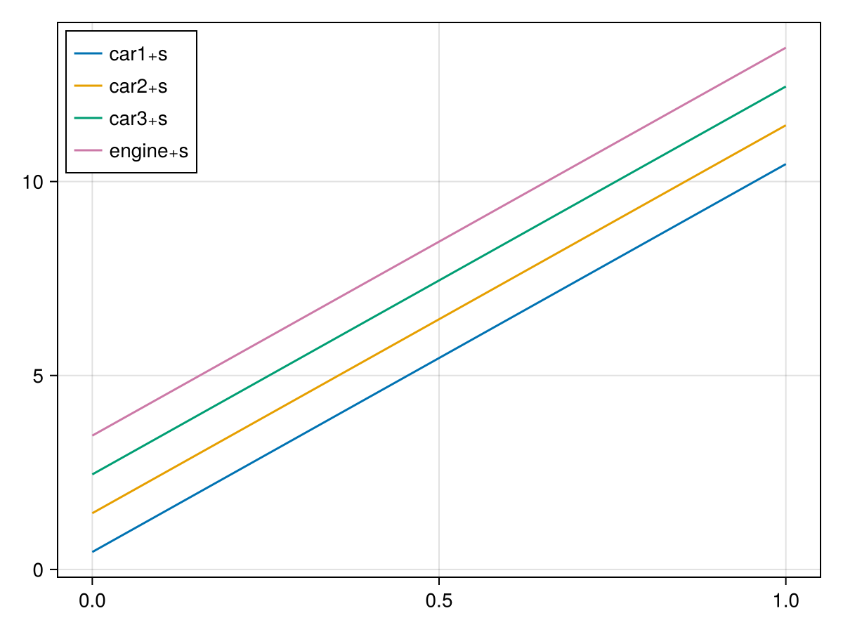

This makes sense! In the absence of any external force, the train should continue to move at a constant velocity, which it does.

Stopper

Now, let's design the stopper,

Building a complete system

Finally, we can unify these two components in a TrainCarWithStopper component.

Let's run this once, without any tuning, to see what happens:

res = TrainCarWithStopperTransientAnalysis()

Transient Analysis Solution for traincar.TrainCarWithStopper
with 8 differential equations and 0 algebraic equations

retcode: Success
Interpolation: 3rd order Hermite
t: 248-element Vector{Float64}: [0.0, 0.25008071291333256 … 9.640764818327135, 10.0]
u: 248-element Vector{Vector{Float64}}:
 [3.45, 2.45, 10.0, 1.45, 10.0, 0.45, 10.0, 10.0]
 [5.95081, 4.95081, 10.0, 3.95081, 10.0, 2.95081, 10.0, 10.0]
 [6.24323, 5.24323, 10.0, 4.24323, 9.99997, 3.24323, 9.99999, 10.0]
 [6.3479, 5.3479, 10.0, 4.3479, 9.99998, 3.3479, 9.99999, 10.0]
 [6.4411, 5.4411, 10.0, 4.4411, 9.99999, 3.4411, 9.99999, 10.0]
 [6.53542, 5.53542, 10.0, 4.53542, 9.99999, 3.53542, 10.0, 10.0]
 [6.63471, 5.63471, 10.0, 4.63471, 10.0, 3.63471, 10.0, 10.0]
 [6.73938, 5.73938, 10.0, 4.73938, 10.0, 3.73938, 10.0, 10.0]
 [6.84767, 5.84767, 10.0, 4.84767, 10.0, 3.84767, 10.0, 10.0]
 [6.95706, 5.95706, 10.0, 4.95706, 10.0, 3.95706, 10.0, 10.0]
 ⋮
 [14.5204, 13.5208, -0.00544766, 12.5211, -0.00590453, 11.5212, -0.00634383, -0.00619935]
 [14.5192, 13.5195, -0.00534571, 12.5197, -0.00570152, 11.5198, -0.00604241, -0.00593044]
 [14.5179, 13.5181, -0.00525964, 12.5183, -0.00553202, 11.5184, -0.00579193, -0.00570668]
 [14.5165, 13.5167, -0.00518794, 12.5168, -0.00539228, 11.5169, -0.0055864, -0.00552283]
 [14.5151, 13.5152, -0.00512911, 12.5153, -0.00527876, 11.5153, -0.00542024, -0.00537399]
 [14.5135, 13.5136, -0.00508167, 12.5136, -0.00518816, 11.5137, -0.00528827, -0.00525561]
 [14.5117, 13.5118, -0.00504415, 12.5118, -0.00511732, 11.5119, -0.00518566, -0.00516342]
 [14.5098, 13.5099, -0.00501511, 12.5099, -0.00506325, 11.5099, -0.00510789, -0.0050934]
 [14.508, 13.5081, -0.00499614, 12.5081, -0.00502856, 11.5081, -0.0050584, -0.00504874]

sol = artifacts(res, :RawSolution)
train_with_stopper = artifacts(res, :SimplifiedSystem)

left_box_idxs = [getproperty(train_with_stopper.cars, Symbol("car", i)).flange_a.s for i in 1:3]
push!(left_box_idxs, train_with_stopper.cars.engine.flange_a.s)
right_box_idxs = [getproperty(train_with_stopper.cars, Symbol("car", i)).flange_b.s for i in 1:3]
push!(right_box_idxs, train_with_stopper.cars.engine.flange_b.s)

t = Observable(0.0)
boxes = lift(t) do t
    starts = sol(t; idxs = left_box_idxs)
    stops = sol(t; idxs = right_box_idxs)
    Rect2f.(tuple.(starts, 0.0), tuple.(stops .- starts, 1.0))
end

f, a, p = poly(boxes)
vlines!(a, 10; color = Makie.Cycled(2), label = "Stopper")
ylims!(a, -4, 5)
xlims!(a, 0, 14)
f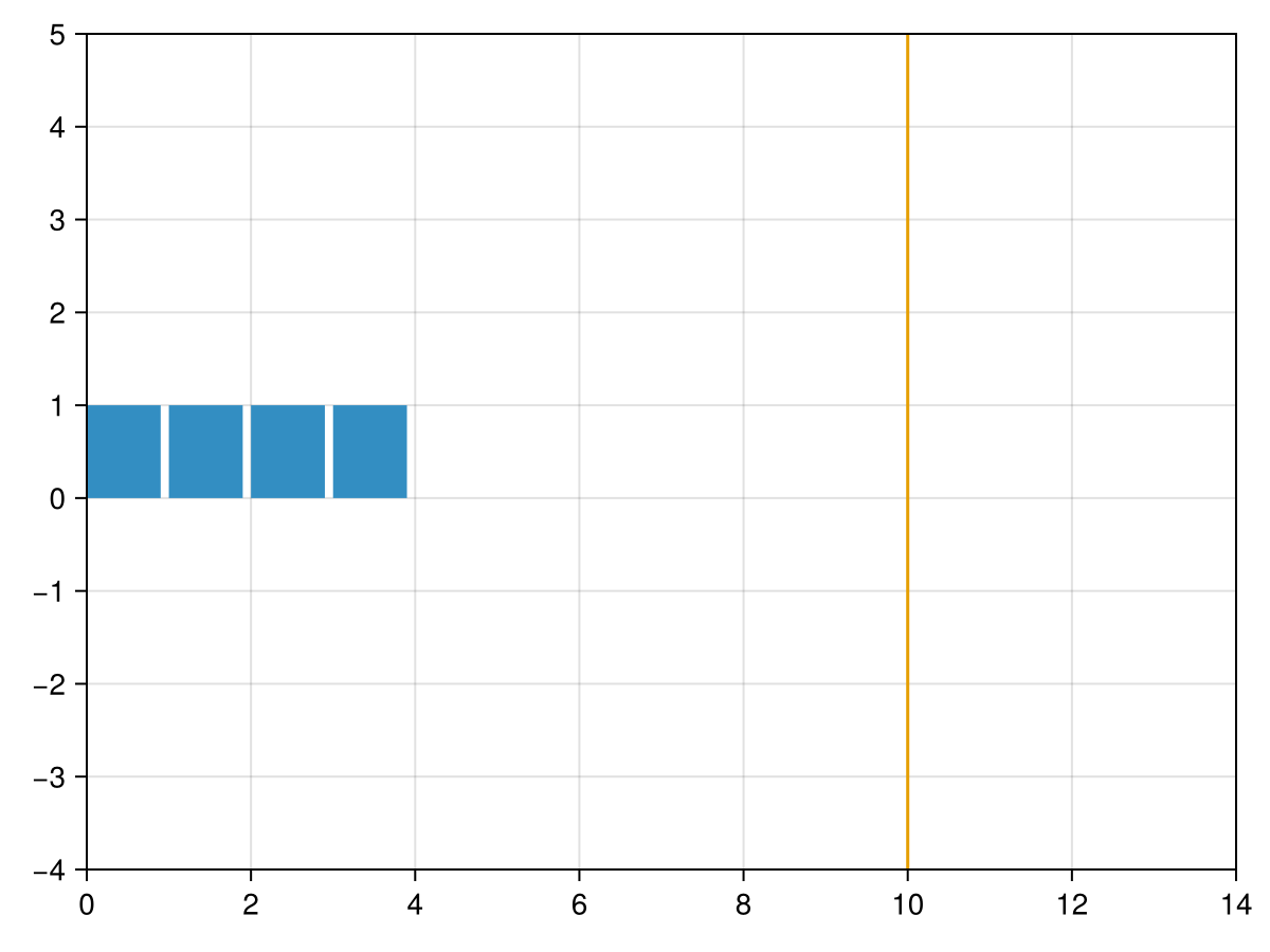

We can also animate this:

record(f, "train_with_stopper.mp4", LinRange(0, 1, 100)) do ti
  t[] = ti
  a.title[] = string("t = ", round(ti; digits = 3))
end

"train_with_stopper.mp4"

Optimizing the System

Now, let's optimize the system to satisfy the design specification.

In order to optimize, we will use the DyadModelOptimizer.jl package, which allows us to optimize a model by specifying an experiment design, constraints, a loss function (running cost), and tunable parameters.

In this case, we will be tuning the spring constant (c) and damping coefficient (d) of the stopper.

using DyadModelOptimizer
using OrdinaryDiffEqRosenbrock: Rodas5P
using ModelingToolkit # to manipulate and construct the Dyad system

First, we need to build the system. The @mtkbuild macro is simply a convenience that will name the system, and structurally simplify it so it can be solved.

@mtkbuild sys = TrainCarWithStopper()

$$\begin{array}{rl}\frac{\mathrm{d}\mathtt{cars}\mathtt{.}\mathtt{engine}\mathtt{.}\mathtt{s}\left(t\right)}{\mathrm{d}t}& =\mathtt{cars}\mathtt{.}\mathtt{engine}\mathtt{.}\mathtt{v}\left(t\right)\\ \frac{\mathrm{d}\mathtt{cars}\mathtt{.}\mathtt{car}\mathtt{3.}\mathtt{s}\left(t\right)}{\mathrm{d}t}& =\mathtt{cars}\mathtt{.}\mathtt{car}\mathtt{3.}\mathtt{v}\left(t\right)\\ \frac{\mathrm{d}\mathtt{cars}\mathtt{.}\mathtt{engine}\mathtt{.}\mathtt{v}\left(t\right)}{\mathrm{d}t}& =\mathtt{cars}\mathtt{.}\mathtt{engine}\mathtt{.}\mathtt{a}\left(t\right)\\ \frac{\mathrm{d}\mathtt{cars}\mathtt{.}\mathtt{car}\mathtt{2.}\mathtt{s}\left(t\right)}{\mathrm{d}t}& =\mathtt{cars}\mathtt{.}\mathtt{car}\mathtt{2.}\mathtt{v}\left(t\right)\\ \frac{\mathrm{d}\mathtt{cars}\mathtt{.}\mathtt{car}\mathtt{3.}\mathtt{v}\left(t\right)}{\mathrm{d}t}& =\mathtt{cars}\mathtt{.}\mathtt{car}\mathtt{3.}\mathtt{a}\left(t\right)\\ \frac{\mathrm{d}\mathtt{cars}\mathtt{.}\mathtt{car}\mathtt{1.}\mathtt{s}\left(t\right)}{\mathrm{d}t}& =\mathtt{cars}\mathtt{.}\mathtt{car}\mathtt{1.}\mathtt{v}\left(t\right)\\ \frac{\mathrm{d}\mathtt{cars}\mathtt{.}\mathtt{car}\mathtt{1.}\mathtt{v}\left(t\right)}{\mathrm{d}t}& =\mathtt{cars}\mathtt{.}\mathtt{car}\mathtt{1.}\mathtt{a}\left(t\right)\\ \frac{\mathrm{d}\mathtt{cars}\mathtt{.}\mathtt{car}\mathtt{2.}\mathtt{v}\left(t\right)}{\mathrm{d}t}& =\mathtt{cars}\mathtt{.}\mathtt{car}\mathtt{2.}\mathtt{a}\left(t\right)\end{array}$$

Now, we define our constraints. We want the acceleration of the last car to be less than 5g, we want the stopper to stop the train before it gets compressed to less than 2 meters, and we want the train to completely stop at the end of the simulation.

In this case, our "loss function", or penalty, is higher the faster the engine is at the end of the simulation period.

We also only want to tune two variables - stopper.c and stopper.d. We allow them to range from 0 to 1,000,000,000 (1e9).

g = 9.807
constraints = [
    -5*g ≲ sys.cars.car3.a
    (sys.stopper.s_a - sys.stopper.s_b) ≲ 2
    0 ≲ sys.cars.engine.v[end]
]

running_cost = abs(sys.cars.engine.v[end]);

tunables = [
    sys.stopper.c => (0, 1e9),
    sys.stopper.d => (0, 1e9),
]

2-element Vector{Pair{Symbolics.Num, Tuple{Int64, Float64}}}:
 stopper₊c => (0, 1.0e9)
 stopper₊d => (0, 1.0e9)

Now that we've defined our constraints and metric of success, we can wrap all of this into a DesignConfiguration, which specifies the experiment design.

Then, we specify the algorithm to use for the optimization. In this case, we will use the SingleShooting algorithm, which is a type of direct collocation method.

Finally. we calibrate the inverse problem and algorithm, and run a simulation.

designconfig = DesignConfiguration(sys;
    alg = Rodas5P(),
    tspan = (0.0, 2.0),
    saveat = 0.0:0.01:2.0,
    constraints = constraints,
    running_cost = running_cost,
    reduction = minimum
)
invprob = InverseProblem(designconfig, tunables)
alg = SingleShooting(maxiters = 1000)
r = calibrate(invprob, alg)
optimized_sol = simulate(designconfig, r)

retcode: Success
Interpolation: 1st order linear
t: 201-element Vector{Float64}:
 0.0
 0.01
 0.02
 0.03
 0.04
 0.05
 0.06
 0.07
 0.08
 0.09
 ⋮
 1.92
 1.93
 1.94
 1.95
 1.96
 1.97
 1.98
 1.99
 2.0
u: 201-element Vector{Vector{Float64}}:
 [3.45, 2.45, 10.0, 1.4500000000000002, 10.0, 0.45, 10.0, 10.0]
 [3.5500000000000007, 2.5500000000000007, 10.0, 1.5500000000000014, 10.0, 0.5500000000000008, 10.0, 9.999999999999998]
 [3.650000000000002, 2.650000000000003, 10.0, 1.650000000000003, 10.0, 0.6500000000000026, 10.0, 10.0]
 [3.750000000000005, 2.7500000000000053, 10.0, 1.7500000000000053, 10.0, 0.7500000000000049, 9.999999999999998, 10.0]
 [3.8500000000000085, 2.8500000000000085, 10.000000000000002, 1.8500000000000083, 10.0, 0.8500000000000081, 10.0, 10.000000000000002]
 [3.950000000000012, 2.950000000000012, 10.0, 1.9500000000000117, 10.0, 0.9500000000000115, 10.0, 10.000000000000002]
 [4.050000000000017, 3.050000000000016, 10.0, 2.0500000000000154, 10.0, 1.0500000000000154, 9.999999999999998, 10.0]
 [4.150000000000022, 3.15000000000002, 10.0, 2.150000000000019, 10.0, 1.1500000000000195, 10.0, 10.000000000000002]
 [4.250000000000026, 3.2500000000000244, 10.0, 2.2500000000000235, 10.0, 1.2500000000000235, 10.0, 10.000000000000002]
 [4.350000000000031, 3.350000000000028, 10.0, 2.3500000000000276, 10.0, 1.3500000000000276, 10.0, 10.000000000000004]
 ⋮
 [11.549723335229137, 10.655981483027833, 0.007740221830810225, 9.72740912097393, -0.09900102248180415, 8.76330127539777, -0.20770261921116354, -0.17124933405819298]
 [11.549794746130322, 10.654989886202388, 0.0065517728627726615, 9.725698028101728, -0.09930837209703752, 8.761227158430998, -0.2071106004734818, -0.1709591398248362]
 [11.549854563229854, 10.653995510626183, 0.0054210593974793235, 9.723990135381342, -0.09955724295241741, 8.759159261829321, -0.2064590888838429, -0.17060982179175602]
 [11.549903351654295, 10.652998926776892, 0.004345627360526694, 9.722286018283066, -0.09975050717325906, 8.757098164003121, -0.2057514000720915, -0.17020454486943812]
 [11.549941652134128, 10.65200067658601, 0.0033231253630559075, 9.72058622082441, -0.0998909127141588, 8.755044410413726, -0.20499070276548165, -0.16974633478419296]
 [11.549969982919219, 10.65100127575423, 0.002351296701021265, 9.718891258164932, -0.0999810931115852, 8.75299851631191, -0.20418003039450916, -0.16923808905477633]
 [11.549988839812574, 10.650001213792189, 0.0014279792141605064, 9.717201616651877, -0.10002356765573488, 8.750960966786035, -0.20332228129737415, -0.16868257718578195]
 [11.549998697353532, 10.649000955449779, 0.0005511003432543933, 9.715517755421464, -0.10002074741463762, 8.748932218451783, -0.2024202258879649, -0.16808244744725237]
 [11.550000009980796, 10.648000942120998, -0.000281327728672743, 9.713840107972722, -0.09997494115573766, 8.746912701112832, -0.20147651370179956, -0.16744023353887083]

We can see from this simulation what the optimal values of c and d are.

Let's plot and animate this optimized system!

sol = optimized_sol

left_box_idxs = [getproperty(sys.cars, Symbol("car", i)).flange_a.s for i in 1:3]
push!(left_box_idxs, sys.cars.engine.flange_a.s)
right_box_idxs = [getproperty(sys.cars, Symbol("car", i)).flange_b.s for i in 1:3]
push!(right_box_idxs, sys.cars.engine.flange_b.s)

t = Observable(0.0)
boxes = lift(t) do t
    starts = sol(t; idxs = left_box_idxs)
    stops = sol(t; idxs = right_box_idxs)
    Rect2f.(tuple.(starts, 0.0), tuple.(stops .- starts, 1.0))
end

f, a, p = poly(boxes)
vlines!(a, 10; color = Makie.Cycled(2), label = "Stopper")
ylims!(a, -4, 5)
xlims!(a, 0, 14)
f

Animating the tuned system

record(f, "optimized_train_with_stopper.mp4", LinRange(0, 1, 100)) do ti
  t[] = ti
  a.title[] = string("t = ", round(ti; digits = 3))
end

"optimized_train_with_stopper.mp4"

Conclusion

In this tutorial, we have shown how to design a stopper for a train using Dyad.