

Examples.TestSlidingModeControl
Test component that validates the SuperTwistingSMC sliding mode controller.
A second-order plant tracks a sinusoidal reference qr = sin(2t) under disturbance d = 2 + 2sin(3t) + sin(5t). The plant position is sampled and differentiated to estimate velocity. The sliding variable s = (xd - qdr) + (x - qr) is computed from the sampled signals and fed to the super-twisting controller. The controller output is held by a ZOH and summed with the disturbance before driving the plant.
SMOKE TEST ONLY. The sign-based sliding-mode switching chatters, so the closed-loop trajectory sits on a switching boundary and is not bit-reproducible across platforms/runners (same SynchToolkit version on a different CPU diverges by up to ~2.16 on secondorder.y). The wide atol/rtol on the test case below therefore only catch gross failures (NaN / unbounded blow-up), NOT trajectory accuracy or regressions. Do not tighten them to "detect regressions" — no pointwise tolerance can survive the platform FP noise here. For real regression coverage, test a platform-stable invariant (e.g. bound/RMS of the sliding variable) instead.
Usage
DiscreteComponents.Examples.TestSlidingModeControl()
Variables
| Name | Description | Units |
|---|---|---|
disturbance | – |
Behavior
Behavior of this component cannot be rendered because it includes path variables.
Source
"""
Test component that validates the SuperTwistingSMC sliding mode controller.

A second-order plant tracks a sinusoidal reference `qr = sin(2t)` under disturbance
`d = 2 + 2sin(3t) + sin(5t)`. The plant position is sampled and differentiated to estimate
velocity. The sliding variable `s = (xd - qdr) + (x - qr)` is computed from the sampled
signals and fed to the super-twisting controller. The controller output is held by a ZOH
and summed with the disturbance before driving the plant.

SMOKE TEST ONLY. The sign-based sliding-mode switching chatters, so the closed-loop
trajectory sits on a switching boundary and is not bit-reproducible across platforms/runners
(same SynchToolkit version on a different CPU diverges by up to ~2.16 on `secondorder.y`).
The wide `atol`/`rtol` on the test case below therefore only catch gross failures
(NaN / unbounded blow-up), NOT trajectory accuracy or regressions. Do not tighten them to
"detect regressions" — no pointwise tolerance can survive the platform FP noise here. For
real regression coverage, test a platform-stable invariant (e.g. bound/RMS of the sliding
variable) instead.
"""
example component TestSlidingModeControl
  # Plant
  secondorder = BlockComponents.Continuous.SecondOrder() {
    "Dyad": {
      "placement": {
        "diagram": {"iconName": "default", "x1": 1020, "y1": 660, "x2": 1120, "y2": 760, "rot": 0}
      },
      "tags": []
    }
  }
  # Velocity estimation via discrete derivative of sampled position
  dd_xd = DiscreteComponents.DiscreteDerivative(initialization = DiscreteComponents.InitialCondition.InitialOutput(y0 = 0.0)) {
    "Dyad": {
      "placement": {
        "diagram": {"iconName": "default", "x1": 140, "y1": 850, "x2": 40, "y2": 950, "rot": 90}
      },
      "tags": []
    }
  }
  # Reference: qr = sin(2t), qdr = 2*cos(2t)
  sine_ref = BlockComponents.Sources.Sine(amplitude = 1, frequency = 0.31831) {
    "Dyad": {
      "placement": {
        "diagram": {"iconName": "default", "x1": -200, "y1": 480, "x2": -100, "y2": 580, "rot": 0}
      },
      "tags": []
    }
  }
  cosine_refd = BlockComponents.Sources.Cosine(amplitude = 2, frequency = 0.31831) {
    "Dyad": {
      "placement": {
        "diagram": {"iconName": "default", "x1": -200, "y1": 690, "x2": -100, "y2": 790, "rot": 0}
      },
      "tags": []
    }
  }
  ps_qr = DiscreteComponents.Sampler() {
    "Dyad": {
      "placement": {
        "diagram": {"iconName": "default", "x1": -70, "y1": 480, "x2": 30, "y2": 580, "rot": 0}
      },
      "tags": []
    }
  }
  ps_qdr = DiscreteComponents.Sampler() {
    "Dyad": {
      "placement": {
        "diagram": {"iconName": "default", "x1": -70, "y1": 690, "x2": 30, "y2": 790, "rot": 0}
      },
      "tags": []
    }
  }
  zoh = DiscreteComponents.ZeroOrderHold() {
    "Dyad": {
      "placement": {
        "diagram": {"iconName": "default", "x1": 690, "y1": 690, "x2": 790, "y2": 790, "rot": 0}
      },
      "tags": []
    }
  }
  # Disturbance: 2 + 2*sin(3t) + sin(5t)
  constant_dist = BlockComponents.Sources.Constant(k = 2) {
    "Dyad": {
      "placement": {
        "diagram": {"iconName": "default", "x1": 520, "y1": 280, "x2": 620, "y2": 380, "rot": 0}
      },
      "tags": []
    }
  }
  sine_dist1 = BlockComponents.Sources.Sine(amplitude = 2, frequency = 0.477465) {
    "Dyad": {
      "placement": {
        "diagram": {"iconName": "default", "x1": 520, "y1": 410, "x2": 620, "y2": 510, "rot": 0}
      },
      "tags": []
    }
  }
  sine_dist2 = BlockComponents.Sources.Sine(amplitude = 1, frequency = 0.795775) {
    "Dyad": {
      "placement": {
        "diagram": {"iconName": "default", "x1": 520, "y1": 540, "x2": 620, "y2": 640, "rot": 0}
      },
      "tags": []
    }
  }
  # Sliding variable computation: s = (x - qr) + (xd_est - qdr)
  err_pos = BlockComponents.Math.Add(k2 = -1) {
    "Dyad": {
      "placement": {
        "diagram": {"iconName": "default", "x1": 150, "y1": 660, "x2": 250, "y2": 560, "rot": 0}
      },
      "tags": []
    }
  }
  err_vel = BlockComponents.Math.Add(k2 = -1) {
    "Dyad": {
      "placement": {
        "diagram": {"iconName": "default", "x1": 150, "y1": 820, "x2": 250, "y2": 720, "rot": 0}
      },
      "tags": []
    }
  }
  """
  sliding surface

  Combines two input signals by multiplying each by its respective gain parameter and adding the results. The output
  is calculated as

  ```math
  y = k1 \cdot u1 + k2 \cdot u2
where k1 and k2 are configurable gain factors that determine the weight of each input in the sum. """ sliding_surface = BlockComponents.Math.Add() { "Dyad": { "placement": { "diagram": {"iconName": "default", "x1": 360, "y1": 690, "x2": 460, "y2": 790, "rot": 0} }, "tags": [] } }
Control + disturbance → plant
add_ctrl = BlockComponents.Math.Add() { "Dyad": { "placement": { "diagram": {"iconName": "default", "x1": 880, "y1": 760, "x2": 980, "y2": 660, "rot": 0} }, "tags": [] } } add3 = BlockComponents.Math.Add3() { "Dyad": { "placement": { "diagram": {"iconName": "default", "x1": 690, "y1": 410, "x2": 790, "y2": 510, "rot": 0} }, "tags": [] } } smc = DiscreteComponents.SuperTwistingSMC(k = 50) { "Dyad": { "placement": { "diagram": {"iconName": "default", "x1": 520, "y1": 690, "x2": 620, "y2": 790, "rot": 0} }, "tags": [] } } periodicclock = DiscreteComponents.PeriodicClock(dt = 0.01) { "Dyad": { "placement": { "diagram": {"iconName": "default", "x1": 880, "y1": 800, "x2": 980, "y2": 900, "rot": 0} }, "tags": [] } } samplewithadeffects = DiscreteComponents.SampleWithADEffects(y_min = -3, y_max = 3, bits = 12, sigma = 0.01) { "Dyad": { "placement": { "diagram": {"iconName": "default", "x1": 980, "y1": 940, "x2": 880, "y2": 1040, "rot": 0} }, "tags": [] } } exponentialfilter = DiscreteComponents.ExponentialFilter(a = 0.2) { "Dyad": { "placement": { "diagram": {"iconName": "default", "x1": 590, "y1": 940, "x2": 490, "y2": 1040, "rot": 0} }, "tags": [] } } variable disturbance::Real relations initial secondorder.x = -1 initial secondorder.xd = 0
Sample references
connect(sine_ref.y, ps_qr.u) {"Dyad": {"edges": [{"S": 1, "M": [], "E": 2}], "renderStyle": "standard"}} connect(cosine_refd.y, ps_qdr.u) {"Dyad": {"edges": [{"S": 1, "M": [], "E": 2}], "renderStyle": "standard"}} connect(zoh.y, add_ctrl.u1) {"Dyad": {"edges": [{"S": 1, "M": [], "E": 2}], "renderStyle": "standard"}} connect(add_ctrl.y, secondorder.u) {"Dyad": {"edges": [{"S": 1, "M": [], "E": 2}], "renderStyle": "standard"}} connect(dd_xd.y, err_vel.u1) { "Dyad": { "edges": [{"S": 1, "M": [{"x": 90, "y": 800}], "E": 2}], "renderStyle": "standard" } } connect(ps_qdr.y, err_vel.u2) {"Dyad": {"edges": [{"S": 1, "M": [], "E": 2}], "renderStyle": "standard"}} connect(err_pos.y, sliding_surface.u1) { "Dyad": { "edges": [{"S": 1, "M": [{"x": 280, "y": 610}, {"x": 280, "y": 710}], "E": 2}], "renderStyle": "standard" } } connect(ps_qr.y, err_pos.u2) { "Dyad": { "edges": [{"S": 1, "M": [{"x": 68, "y": 530}, {"x": 68, "y": 580}], "E": 2}], "renderStyle": "standard" } } connect(sine_dist1.y, add3.u2) {"Dyad": {"edges": [{"S": 1, "M": [], "E": 2}], "renderStyle": "standard"}} connect(add3.y, add_ctrl.u2) { "Dyad": { "edges": [{"S": 1, "M": [{"x": 830, "y": 460}, {"x": 830, "y": 680}], "E": 2}], "renderStyle": "standard" } } connect(err_vel.y, sliding_surface.u2) {"Dyad": {"renderStyle": "standard", "edges": [{"S": 1, "E": 2, "M": []}]}} connect(smc.s, sliding_surface.y) {"Dyad": {"edges": [{"S": 1, "M": [], "E": 2}], "renderStyle": "standard"}} connect(smc.y, zoh.u) {"Dyad": {"edges": [{"S": 1, "M": [], "E": 2}], "renderStyle": "standard"}} connect(constant_dist.y, add3.u1) { "Dyad": { "renderStyle": "standard", "edges": [{"S": 1, "M": [{"x": 657.5, "y": 330}, {"x": 657.5, "y": 430}], "E": 2}] } } connect(sine_dist2.y, add3.u3) { "Dyad": { "renderStyle": "standard", "edges": [{"S": 1, "M": [{"x": 657.5, "y": 590}, {"x": 657.5, "y": 490}], "E": 2}] } } connect(samplewithadeffects.y, periodicclock.y, exponentialfilter.u) { "Dyad": { "edges": [ {"S": 1, "M": [], "E": -1}, {"S": -1, "M": [{"x": 810, "y": 990}, {"x": 810, "y": 850}], "E": 2}, {"S": 3, "M": [], "E": -1} ], "junctions": [{"x": 810, "y": 990}], "renderStyle": "standard" } } connect(samplewithadeffects.u, secondorder.y) { "Dyad": { "edges": [{"S": 1, "M": [{"x": 1160, "y": 990}, {"x": 1160, "y": 710}], "E": 2}], "renderStyle": "standard" } } connect(exponentialfilter.y, dd_xd.u, err_pos.u1) { "Dyad": { "edges": [ {"S": 1, "M": [], "E": -1}, {"S": -1, "M": [], "E": 2}, {"S": 3, "M": [{"x": -270, "y": 640}, {"x": -270, "y": 990}], "E": -1} ], "junctions": [{"x": 90, "y": 990}], "renderStyle": "standard" } } metadata { "Dyad": { "tests": { "case1": { "stop": 6, "atol": {"secondorder.y": 2.5, "smc.y": 0.1}, "rtol": {"secondorder.y": 0.5, "smc.y": 0.05}, "expect": {"signals": ["secondorder.y", "smc.y"]} } }, "doc": {"behavior": false} } } end
<details>
<summary>Flattened Source</summary>


```dyad
"""
Test component that validates the SuperTwistingSMC sliding mode controller.

A second-order plant tracks a sinusoidal reference `qr = sin(2t)` under disturbance
`d = 2 + 2sin(3t) + sin(5t)`. The plant position is sampled and differentiated to estimate
velocity. The sliding variable `s = (xd - qdr) + (x - qr)` is computed from the sampled
signals and fed to the super-twisting controller. The controller output is held by a ZOH
and summed with the disturbance before driving the plant.

SMOKE TEST ONLY. The sign-based sliding-mode switching chatters, so the closed-loop
trajectory sits on a switching boundary and is not bit-reproducible across platforms/runners
(same SynchToolkit version on a different CPU diverges by up to ~2.16 on `secondorder.y`).
The wide `atol`/`rtol` on the test case below therefore only catch gross failures
(NaN / unbounded blow-up), NOT trajectory accuracy or regressions. Do not tighten them to
"detect regressions" — no pointwise tolerance can survive the platform FP noise here. For
real regression coverage, test a platform-stable invariant (e.g. bound/RMS of the sliding
variable) instead.
"""
example component TestSlidingModeControl
  # Plant
  secondorder = BlockComponents.Continuous.SecondOrder() {
    "Dyad": {
      "placement": {
        "diagram": {"iconName": "default", "x1": 1020, "y1": 660, "x2": 1120, "y2": 760, "rot": 0}
      },
      "tags": []
    }
  }
  # Velocity estimation via discrete derivative of sampled position
  dd_xd = DiscreteComponents.DiscreteDerivative(initialization = DiscreteComponents.InitialCondition.InitialOutput(y0 = 0.0)) {
    "Dyad": {
      "placement": {
        "diagram": {"iconName": "default", "x1": 140, "y1": 850, "x2": 40, "y2": 950, "rot": 90}
      },
      "tags": []
    }
  }
  # Reference: qr = sin(2t), qdr = 2*cos(2t)
  sine_ref = BlockComponents.Sources.Sine(amplitude = 1, frequency = 0.31831) {
    "Dyad": {
      "placement": {
        "diagram": {"iconName": "default", "x1": -200, "y1": 480, "x2": -100, "y2": 580, "rot": 0}
      },
      "tags": []
    }
  }
  cosine_refd = BlockComponents.Sources.Cosine(amplitude = 2, frequency = 0.31831) {
    "Dyad": {
      "placement": {
        "diagram": {"iconName": "default", "x1": -200, "y1": 690, "x2": -100, "y2": 790, "rot": 0}
      },
      "tags": []
    }
  }
  ps_qr = DiscreteComponents.Sampler() {
    "Dyad": {
      "placement": {
        "diagram": {"iconName": "default", "x1": -70, "y1": 480, "x2": 30, "y2": 580, "rot": 0}
      },
      "tags": []
    }
  }
  ps_qdr = DiscreteComponents.Sampler() {
    "Dyad": {
      "placement": {
        "diagram": {"iconName": "default", "x1": -70, "y1": 690, "x2": 30, "y2": 790, "rot": 0}
      },
      "tags": []
    }
  }
  zoh = DiscreteComponents.ZeroOrderHold() {
    "Dyad": {
      "placement": {
        "diagram": {"iconName": "default", "x1": 690, "y1": 690, "x2": 790, "y2": 790, "rot": 0}
      },
      "tags": []
    }
  }
  # Disturbance: 2 + 2*sin(3t) + sin(5t)
  constant_dist = BlockComponents.Sources.Constant(k = 2) {
    "Dyad": {
      "placement": {
        "diagram": {"iconName": "default", "x1": 520, "y1": 280, "x2": 620, "y2": 380, "rot": 0}
      },
      "tags": []
    }
  }
  sine_dist1 = BlockComponents.Sources.Sine(amplitude = 2, frequency = 0.477465) {
    "Dyad": {
      "placement": {
        "diagram": {"iconName": "default", "x1": 520, "y1": 410, "x2": 620, "y2": 510, "rot": 0}
      },
      "tags": []
    }
  }
  sine_dist2 = BlockComponents.Sources.Sine(amplitude = 1, frequency = 0.795775) {
    "Dyad": {
      "placement": {
        "diagram": {"iconName": "default", "x1": 520, "y1": 540, "x2": 620, "y2": 640, "rot": 0}
      },
      "tags": []
    }
  }
  # Sliding variable computation: s = (x - qr) + (xd_est - qdr)
  err_pos = BlockComponents.Math.Add(k2 = -1) {
    "Dyad": {
      "placement": {
        "diagram": {"iconName": "default", "x1": 150, "y1": 660, "x2": 250, "y2": 560, "rot": 0}
      },
      "tags": []
    }
  }
  err_vel = BlockComponents.Math.Add(k2 = -1) {
    "Dyad": {
      "placement": {
        "diagram": {"iconName": "default", "x1": 150, "y1": 820, "x2": 250, "y2": 720, "rot": 0}
      },
      "tags": []
    }
  }
  """
  sliding surface

  Combines two input signals by multiplying each by its respective gain parameter and adding the results. The output
  is calculated as

  ```math
  y = k1 \cdot u1 + k2 \cdot u2
where k1 and k2 are configurable gain factors that determine the weight of each input in the sum. """ sliding_surface = BlockComponents.Math.Add() { "Dyad": { "placement": { "diagram": {"iconName": "default", "x1": 360, "y1": 690, "x2": 460, "y2": 790, "rot": 0} }, "tags": [] } }
Control + disturbance → plant
add_ctrl = BlockComponents.Math.Add() { "Dyad": { "placement": { "diagram": {"iconName": "default", "x1": 880, "y1": 760, "x2": 980, "y2": 660, "rot": 0} }, "tags": [] } } add3 = BlockComponents.Math.Add3() { "Dyad": { "placement": { "diagram": {"iconName": "default", "x1": 690, "y1": 410, "x2": 790, "y2": 510, "rot": 0} }, "tags": [] } } smc = DiscreteComponents.SuperTwistingSMC(k = 50) { "Dyad": { "placement": { "diagram": {"iconName": "default", "x1": 520, "y1": 690, "x2": 620, "y2": 790, "rot": 0} }, "tags": [] } } periodicclock = DiscreteComponents.PeriodicClock(dt = 0.01) { "Dyad": { "placement": { "diagram": {"iconName": "default", "x1": 880, "y1": 800, "x2": 980, "y2": 900, "rot": 0} }, "tags": [] } } samplewithadeffects = DiscreteComponents.SampleWithADEffects(y_min = -3, y_max = 3, bits = 12, sigma = 0.01) { "Dyad": { "placement": { "diagram": {"iconName": "default", "x1": 980, "y1": 940, "x2": 880, "y2": 1040, "rot": 0} }, "tags": [] } } exponentialfilter = DiscreteComponents.ExponentialFilter(a = 0.2) { "Dyad": { "placement": { "diagram": {"iconName": "default", "x1": 590, "y1": 940, "x2": 490, "y2": 1040, "rot": 0} }, "tags": [] } } variable disturbance::Real relations initial secondorder.x = -1 initial secondorder.xd = 0
Sample references
connect(sine_ref.y, ps_qr.u) {"Dyad": {"edges": [{"S": 1, "M": [], "E": 2}], "renderStyle": "standard"}} connect(cosine_refd.y, ps_qdr.u) {"Dyad": {"edges": [{"S": 1, "M": [], "E": 2}], "renderStyle": "standard"}} connect(zoh.y, add_ctrl.u1) {"Dyad": {"edges": [{"S": 1, "M": [], "E": 2}], "renderStyle": "standard"}} connect(add_ctrl.y, secondorder.u) {"Dyad": {"edges": [{"S": 1, "M": [], "E": 2}], "renderStyle": "standard"}} connect(dd_xd.y, err_vel.u1) { "Dyad": { "edges": [{"S": 1, "M": [{"x": 90, "y": 800}], "E": 2}], "renderStyle": "standard" } } connect(ps_qdr.y, err_vel.u2) {"Dyad": {"edges": [{"S": 1, "M": [], "E": 2}], "renderStyle": "standard"}} connect(err_pos.y, sliding_surface.u1) { "Dyad": { "edges": [{"S": 1, "M": [{"x": 280, "y": 610}, {"x": 280, "y": 710}], "E": 2}], "renderStyle": "standard" } } connect(ps_qr.y, err_pos.u2) { "Dyad": { "edges": [{"S": 1, "M": [{"x": 68, "y": 530}, {"x": 68, "y": 580}], "E": 2}], "renderStyle": "standard" } } connect(sine_dist1.y, add3.u2) {"Dyad": {"edges": [{"S": 1, "M": [], "E": 2}], "renderStyle": "standard"}} connect(add3.y, add_ctrl.u2) { "Dyad": { "edges": [{"S": 1, "M": [{"x": 830, "y": 460}, {"x": 830, "y": 680}], "E": 2}], "renderStyle": "standard" } } connect(err_vel.y, sliding_surface.u2) {"Dyad": {"renderStyle": "standard", "edges": [{"S": 1, "E": 2, "M": []}]}} connect(smc.s, sliding_surface.y) {"Dyad": {"edges": [{"S": 1, "M": [], "E": 2}], "renderStyle": "standard"}} connect(smc.y, zoh.u) {"Dyad": {"edges": [{"S": 1, "M": [], "E": 2}], "renderStyle": "standard"}} connect(constant_dist.y, add3.u1) { "Dyad": { "renderStyle": "standard", "edges": [{"S": 1, "M": [{"x": 657.5, "y": 330}, {"x": 657.5, "y": 430}], "E": 2}] } } connect(sine_dist2.y, add3.u3) { "Dyad": { "renderStyle": "standard", "edges": [{"S": 1, "M": [{"x": 657.5, "y": 590}, {"x": 657.5, "y": 490}], "E": 2}] } } connect(samplewithadeffects.y, periodicclock.y, exponentialfilter.u) { "Dyad": { "edges": [ {"S": 1, "M": [], "E": -1}, {"S": -1, "M": [{"x": 810, "y": 990}, {"x": 810, "y": 850}], "E": 2}, {"S": 3, "M": [], "E": -1} ], "junctions": [{"x": 810, "y": 990}], "renderStyle": "standard" } } connect(samplewithadeffects.u, secondorder.y) { "Dyad": { "edges": [{"S": 1, "M": [{"x": 1160, "y": 990}, {"x": 1160, "y": 710}], "E": 2}], "renderStyle": "standard" } } connect(exponentialfilter.y, dd_xd.u, err_pos.u1) { "Dyad": { "edges": [ {"S": 1, "M": [], "E": -1}, {"S": -1, "M": [], "E": 2}, {"S": 3, "M": [{"x": -270, "y": 640}, {"x": -270, "y": 990}], "E": -1} ], "junctions": [{"x": 90, "y": 990}], "renderStyle": "standard" } } metadata { "Dyad": { "tests": { "case1": { "stop": 6, "atol": {"secondorder.y": 2.5, "smc.y": 0.1}, "rtol": {"secondorder.y": 0.5, "smc.y": 0.05}, "expect": {"signals": ["secondorder.y", "smc.y"]} } }, "doc": {"behavior": false} } } end
</details>


<br></br>


## Test Cases {#Test-Cases}

### Test Case `case1` {#Test-Case-case1}

```julia
plt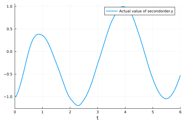
plt
Related
Examples
Experiments
Analyses