Building an Inversion-Based Controller
In this tutorial we will model and simulate an active suspension model using components from our standard libraries.
To get started, create a new component library, as indicated on the Getting started page.
The Active Suspension Model
We will use components from our standard libraries: DyadExampleComponents, TranslationalComponents, and BlockComponents. Additionally, we will import DyadControlSystems. In the Julia REPL, run the following commands:
using Pkg
Pkg.add(["DyadExampleComponents", "TranslationalComponents", "BlockComponents", "DyadControlSystems"])
Schematic in Dyad Builder

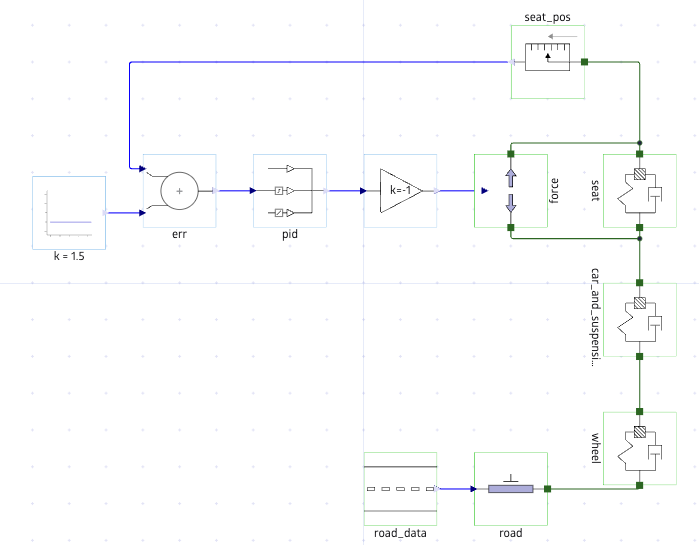
The above schematic is the graphical representation of the ActiveSuspension model in Dyad Builder. It represents a vehicle moving over a bumpy road. On the vehicle is a PID controller controlling an actuating force which dampens the seat response to the reference position of 1.5. The vehicle consists of a seat, suspension system, and wheel. Each of these three elements is modeled as a MassSpringDamper from the DyadExampleComponents library.
Let's define this model in our library. In the dyad folder, create a new file named ActiveSuspension.dyad and include the code below.
component ActiveSuspension
  wheel = DyadExampleComponents.MassSpringDamper(m = wheel_mass, d = wheel_damping, c = wheel_stiffness, g = -10, theta = pi / 2) {^wheel}
  car_and_suspension = DyadExampleComponents.MassSpringDamper(m = car_mass, d = suspension_damping, c = suspension_stiffness, g = -10, theta = pi / 2) {^car_and_suspension}
  seat = DyadExampleComponents.MassSpringDamper(m = human_and_seat_mass, d = seat_damping, c = seat_stiffness, g = -10, theta = pi / 2) {^seat}
  road_data = DyadExampleComponents.RoadData() {^road_data}
  road = DyadExampleComponents.SimplePosition() {^road}
  force = TranslationalComponents.Force() {^force}
  pid = BlockComponents.LimPID(k = Kp, Ti = Ti, Td = Td) {^pid}
  set_point = BlockComponents.Constant(k = 1.5) {^set_point}
  seat_pos = TranslationalComponents.PositionSensor() {^seat_pos}
  parameter wheel_mass::Dyad.Mass = 25
  parameter wheel_stiffness::TranslationalSpringConstant = 1e2
  parameter wheel_damping::DampingCoefficient = 1e4
  parameter car_mass::Dyad.Mass = 1000
  parameter suspension_stiffness::TranslationalSpringConstant = 1e4
  parameter suspension_damping::DampingCoefficient = 10
  parameter human_and_seat_mass::Dyad.Mass = 100
  parameter seat_stiffness::TranslationalSpringConstant = 1000
  parameter seat_damping::DampingCoefficient = 1
  parameter wheel_initial_position::Dyad.Position = 0.5
  parameter suspension_initial_position::Dyad.Position = 1
  parameter seat_initial_position::Dyad.Position = 1.5
  parameter Kp::Real = 20
  parameter Ti::Real = 5
  parameter Td::Real = 1
relations
  initial wheel.mass.s = wheel_initial_position
  initial car_and_suspension.mass.s = suspension_initial_position
  initial seat.mass.s = seat_initial_position
  initial wheel.mass.v = 0
  initial car_and_suspension.mass.v = 0
  initial seat.mass.v = 0
  initial wheel.mass.a = 0
  initial car_and_suspension.mass.a = 0
  initial seat.mass.a = 0
  u: analysis_point(pid.y, force.f)
  y: analysis_point(seat_pos.s, pid.u_m)
  pid.u_ff = 0
  connect(wheel.flange_sd, road.flange)
  connect(car_and_suspension.flange_sd, wheel.flange_m)
  connect(car_and_suspension.flange_m, seat.flange_sd, force.flange_a)
  connect(seat.flange_m, force.flange_b, seat_pos.flange)
  connect(pid.y, force.f)
  connect(pid.u_s, set_point.y)
  connect(seat_pos.s, pid.u_m)
  connect(road_data.y, road.s)
end
To simulate this model, we create an analysis that extends the TransientAnalysis type and uses our ActiveSuspension model:
analysis ActiveSuspensionTransient
  extends TransientAnalysis(alg=ODEAlg.Auto(), abstol=10m, reltol=1m, start=0, stop=10)
  model = ActiveSuspension()
end
Let's run this analysis and plot two signals: the seat position and force response. Run the following commands in the Julia REPL:
# using <LibraryName>
using ModelingToolkit
using Plots
using DyadInterface

sol1 = ActiveSuspensionTransient()
as = artifacts(sol1, :SimplifiedSystem)

plot(sol1, idxs = [as.seat_pos.s],
  title = "Seat position",
  xlabel = "Time (sec)",
  ylabel = "Position"
)
plot(sol1, idxs = [as.force.f],
  title = "Force supplied by actuator",
  xlabel = "Time (sec)",
  ylabel = "Force (N)"
)
Tuning the Controller
The controller in the above model is not tuned. We can specify another analysis to tune the controller. Since the PID autotuning analysis internally opens the loop at the measurement point y, the connection from seat_pos.s to pid.u_m is broken during linearization. We need to provide an initial condition for pid.u_m so that the operating point is well-defined:
component ActiveSuspensionForAutotuning
  extends ActiveSuspension()
relations
  initial pid.u_m = 1.5
end

analysis ActiveSuspensionPIDAutotuningAnalysis
  extends DyadControlSystems.PIDAutotuningAnalysis(
    measurement = "y",
    control_input = "u",
    step_input = "u",
    step_output = "y",
    Ts = 0.01,
    duration = 10.0,
    Ms = 1.2,
    Mt = 1.1,
    Mks = 3e4,
    ki_lb = 2000,
    wl = 1e-2,
    wu = 1e3
  )
  model = ActiveSuspensionForAutotuning()
end
Once we specify the analysis declaratively, we can run it imperatively:
using DyadInterface
using Plots
sol = ActiveSuspensionPIDAutotuningAnalysis()
PID Autotuning Analysis solution for PIDAutotuningAnalysis
Optimized parameters (parallel form): [763.1073446297678, 5431.9891078208675, 714.3126666827111, 0.026504673820710346]
Cost: 9.001960976281153e-8
Disk-based margins:
Gain margins: 0.2, 5.3
Phase margin: 68.7°
Delay margin: 0.07277380397091959sWe may plot some of the available artifacts:
figs  = artifacts(sol, :SensitivityFunctions)
fign  = artifacts(sol, :NoiseSensitivityAndController)
figr  = artifacts(sol, :OptimizedResponse)
figny = artifacts(sol, :NyquistPlot)

plot!(figs, ylims=(1e-2, Inf))
plot!(figny, legend=:bottomleft)

plot(figs, fign, figr, figny,
    link = :none,
    size = (600, 600),
)
We may also ask for the optimized controller parameters:
artifacts(sol, :OptimizedParameters)| Row | kp_parallel | ki_parallel | kd_parallel | Kp_standard | Ti_standard | Td_standard | Tf |
|---|---|---|---|---|---|---|---|
| Float64 | Float64 | Float64 | Float64 | Float64 | Float64 | Float64 | |
| 1 | 763.107 | 5431.99 | 714.313 | 763.107 | 0.140484 | 0.936058 | 0.0265047 |
Inverting the Model
Say we need to know the force requirement of the actuator if the control system were to keep the seat position precisely at the reference value of 1.5 as the vehicle moves over the bumpy road. In many workflows, we would first need to autotune the PID controller to determine the appropriate controller gain values before we are able to calculate the corresponding force signal. In a acausal modeling framework like Dyad, however, we are able to solve for the force signal directly without having to tune the PID controller.
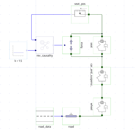
To do this, we will create a component, ReverseCausality, that extends from the SI2SO component from the BlockComponents library. ReverseCausality will constrain its inputs to be equal to one another. This will allow us to constrain the seat position to the reference value in our model. When we simulate, the model will then calculate all other signals such that this constraint is met. Another way to think of it: rather than having the PID controller drive the actuating force based on the PID gains, we will have the ReverseCausality block drive the actuating force based on the constraint that the two block inputs must be equal to one another.
In the dyad folder, create a new file named InvertedActiveSuspension.dyad and include the code below.
component ReverseCausality
    extends BlockComponents.SI2SO
relations
    u1 = u2
end
Schematic in Dyad GUI

We will modify our model to remove the PID controller and incorporate the ReverseCausality component, see the schematic above for the graphical representation of this in Dyad Builder. Below is the Dyad implementation for this InvertedActiveSuspension model, include it in the InvertedActiveSuspension.dyad file:
component InvertedActiveSuspension
  wheel = DyadExampleComponents.MassSpringDamper(m = wheel_mass, d = wheel_damping, c = wheel_stiffness, g = -10, theta = pi / 2) {^wheel}
  car_and_suspension = DyadExampleComponents.MassSpringDamper(m = car_mass, d = suspension_damping, c = suspension_stiffness, g = -10, theta = pi / 2) {^car_and_suspension}
  seat = DyadExampleComponents.MassSpringDamper(m = human_and_seat_mass, d = seat_damping, c = seat_stiffness, g = -10, theta = pi / 2) {^seat}
  road_data = DyadExampleComponents.RoadData() {^road_data}
  rev_causality = ReverseCausality() {^rev_causality}
  road = DyadExampleComponents.SimplePosition() {^road}
  force = TranslationalComponents.Force() {^force}
  set_point = BlockComponents.Constant(k = 1.5) {^set_point}
  seat_pos = TranslationalComponents.PositionSensor() {^seat_pos}
  parameter wheel_mass::Dyad.Mass = 25
  parameter wheel_stiffness::TranslationalSpringConstant = 1e2
  parameter wheel_damping::DampingCoefficient = 1e4
  parameter car_mass::Dyad.Mass = 1000
  parameter suspension_stiffness::TranslationalSpringConstant = 1e4
  parameter suspension_damping::DampingCoefficient = 10
  parameter human_and_seat_mass::Dyad.Mass = 100
  parameter seat_stiffness::TranslationalSpringConstant = 1000
  parameter seat_damping::DampingCoefficient = 1
  parameter wheel_initial_position::Dyad.Position = 0.5
  parameter suspension_initial_position::Dyad.Position = 1
  parameter seat_initial_position::Dyad.Position = 1.5
  parameter kd::Real = 20
  parameter ki::Real = 0.2
  parameter kp::Real = 1
relations
  initial wheel.mass.s = wheel_initial_position
  initial car_and_suspension.mass.s = suspension_initial_position
  initial wheel.mass.v = 0
  initial car_and_suspension.mass.v = 0
  initial wheel.mass.a = 0
  initial car_and_suspension.mass.a = 0
  initial force.f = 0
  connect(wheel.flange_sd, road.flange) {^id10}
  connect(car_and_suspension.flange_sd, wheel.flange_m) {^id11}
  connect(car_and_suspension.flange_m, seat.flange_sd, force.flange_a) {^id12}
  connect(seat.flange_m, force.flange_b, seat_pos.flange) {^id13}
  connect(seat_pos.s, rev_causality.u1) {^id14}
  connect(rev_causality.u2, set_point.y) {^id15}
  connect(force.f, rev_causality.y) {^id16}
  connect(road_data.y, road.s) {^id17}
end
Similarly to before, we create an analysis that extends the TransientAnalysis type and uses our InvertedActiveSuspension model:
analysis InvertedActiveSuspensionTransient
  extends TransientAnalysis(alg=ODEAlg.Auto(), abstol=10m, reltol=1m, start=0, stop=10)
  model = InvertedActiveSuspension()
end
Finally, we can compare the seat positions and force responses between the nominal and the inverted models:
using ModelingToolkit
using Plots
using DyadInterface

sol1 = ActiveSuspensionTransient()
as = artifacts(sol1, :SimplifiedSystem)

sol2 = InvertedActiveSuspensionTransient()
ias = artifacts(sol2, :SimplifiedSystem)

plot(sol1, idxs = [as.seat_pos.s],
  title = "Seat position",
  label = "Baseline Model",
  xlabel = "Time (sec)",
  ylabel = "Position"
)
plot!(sol2, idxs = [ias.seat_pos.s],
  label = "Inverted Model",
  xlabel = "Time (sec)",
  ylabel = "Position"
)

plot(sol1, idxs = [as.force.f],
  title = "Force supplied by actuator",
  label = "Baseline Model",
  xlabel = "Time (sec)",
  ylabel = "Force (N)"
)
plot!(sol2, idxs = [ias.force.f],
  label = "Inverted Model",
  xlabel = "Time (sec)",
  ylabel = "Force (N)"
)