
Discrete-Time Modeling
Dyad models discrete-time behaviour with clocks. A clock is an event source: when it ticks, the discrete-time logic associated with it runs once. Variables that only have a value at the ticks of a clock are called clocked, and the equations relating them are difference equations rather than differential equations.
Nothing on this page requires a continuous-time part. A model can be entirely discrete-time — a filter chain, a supervisory state machine, a controller you intend to deploy on its own. When a discrete-time model is combined with a continuous-time one, the result is a sampled-data system, which adds a small number of further concerns; those are covered in Sampled-Data Systems.
The synchronous programming model
Discrete-time models in Dyad follow the synchronous model of computation:
Computation takes no time. Everything that happens at a tick — every equation in that clock's partition — happens at a single instant of model time. A chain of ten blocks costs no more model time than one block.
Communication takes no time. A value produced at a tick is available to every other equation on the same clock at that same tick. There is no transport delay unless you explicitly model one.
Each tick completes before the next begins. There is no overlap between one tick's computation and the next, so a partition never sees a half-updated state.
Delay is explicit. Because computation is instantaneous, the only way a value becomes "old" is if you ask for an earlier one, with
x@(clk-1).
The consequence to keep in mind is that model time and execution time are different things. If the generated program takes longer to run than the clock period on real hardware, the model will not have predicted it and it may behave in unintended ways.
Clocks and partitions
Any variable appearing in an equation with a clocked variable is inferred to belong to the same discrete-time partition — the set of variables sharing one clock. A model may contain several partitions, each with its own clock, which is how multi-rate systems and logic distributed across several computers are expressed.
Clock sources
Every discrete-time partition needs a clock source to tell it when to tick. The available sources and clock-plumbing components are:
| Component | Purpose |
|---|---|
PeriodicClock | Ticks every dt time units. The workhorse — connect its y connector to any signal in the partition you want to clock. |
ZeroCrossingClock | An event clock that ticks when its continuous input crosses zero, rather than on a fixed schedule. |
SampleTimeSource | Outputs the sample interval of its clock as a signal, for logic that needs it as a value rather than as a parameter. |
LastValue | Carries a signal from one clock to another by taking the last value it had. Cheaper than a ZeroOrderHold followed by a Sampler. |
ClockPropagator | Experimental. Forces two signals onto the same clock without relating their values. |
PeriodicClock has no default dt
dt is a structural parameter with no default, so it must always be supplied. Omitting it fails with UndefKeywordError: keyword argument dt not assigned.
A partition needs one clock, but not necessarily one clock component: two PeriodicClocks with the same dt are treated as synchronised and merge into a single partition. A model may therefore legitimately declare a clock next to each of several blocks that run at the same rate, as the cascade example does. Clocks with different rates always form separate partitions.
Clock syntax
Dyad uses the @clk and @(clk-n) syntax to refer to current and past values of discrete-time variables. For the full grammar of clock annotations, see Clocks in the syntax manual. The example below illustrates the Dyad clock syntax, implementing the discrete-time system
In Dyad, this is written with negative shifts (all indices shifted by -1):
x@clk = 0.5 * x@(clk-1) + u@(clk-1)
y = x
A few things to note in this basic example:
The equation
xanduare automatically inferred to be discrete-time variables, since they appear in an equation with a clock annotation@clk.yis also automatically inferred to be a discrete-time variable, since it appears in an equation with another discrete-time variablex. All variablesx, u, ybelong to the same discrete-time partition.The equation
y = xdoes not use any clock annotation — this is equivalent toy@clk = x@clk, i.e., discrete-time variables without clock annotations are assumed to refer to the variable at the current time step.The equation
x@clk = 0.5 * x@(clk-1) + u@(clk-1)indicates howxis updated: the value ofxat the current time step is computed in terms of past values. If this logic was implemented in an imperative programming style, the logic would be:
function discrete_step(x, u)
    x = 0.5x + u  # x is updated to a new value, i.e., x(k) is computed
    y = x         # y is assigned the current value of x, y(k) = x(k)
    return x, y
end
Note that the following system is not equivalent to the one above:
x@clk = 0.5 * x@(clk-1) + u@clk
y = x
In this version, u@clk refers to the input at the current time point, making the system equivalent to
Higher-order shifts
The expression x@(clk-1) refers to the value of x at the previous clock tick. Similarly, x@(clk-2) refers to the value of x at the clock tick before that. In general, x@(clk-n) refers to the value of x at the nth clock tick before the current one. As an example, the Z-domain transfer function
may be modeled in Dyad as
y@clk = (b2 * u@clk + b1 * u@(clk-1) + b0 * u@(clk-2) - a1 * y@(clk-1) - a0 * y@(clk-2)) / a2or using the DiscreteTransferFunction component with numerator and denominator coefficient arrays.
Clocked equations must be explicit
Unlike continuous-time equations, which may be written in implicit acausal form, a clocked equation must be an assignment: the left-hand side has to be a single variable at the current tick. The recurrence above therefore has to be solved for y@clk by hand. Writing it implicitly,
a2 * y@clk + a1 * y@(clk-1) + a0 * y@(clk-2) = b2 * u@clk + b1 * u@(clk-1) + b0 * u@(clk-2)is not supported.
Initial conditions
The initial condition of discrete-time variables is specified using the initial keyword with a past clock reference, for example:
initial x@(clk-1) = 1.0Note how the initial condition for discrete-time variables refers to the past. The reason is that in order to perform the discrete-time state update
If higher-order shifts are present, the corresponding initial conditions must be specified. For example, a component using x@(clk-2) requires both:
initial x@(clk-1) = 0.0
initial x@(clk-2) = 0.0
When building test components, initial conditions for subcomponent states are specified in the relations block. For instance, initial secondorder.x = 0.0 sets the initial condition of a subcomponent's continuous-time state.
Multiple clocks
Multi-rate systems are modeled using multiple PeriodicClock components with different dt values. Each distinct rate defines its own discrete-time partition, so signals in each partition are updated at the corresponding rate. This is how you model, for example, a fast inner control loop and a slow outer loop, or discrete-time processes running on different computers.
A signal cannot be used directly across two partitions with different rates — the compiler reports Attempted to combine two independent (output) clocks or a clock conflict. Use LastValue to carry a value from one clock to another; it places the most recent value of its input onto its output's clock.
The example below samples the same sine wave on a fast (20 Hz) and a slow (4 Hz) clock, and uses LastValue to bring the fast signal into the slow partition. Download as a Dyad projectmultirate.zipOpen in Dyad Studio
"""
Two discrete-time partitions at different rates. The fast partition samples the source
at 20 Hz; `LastValue` carries the fast signal into the 4 Hz slow partition.
"""
test component MultiRateDemo
  source = BlockComponents.Sources.Sine(amplitude = 1, frequency = 1)
  "Fast partition: 20 Hz"
  fast_sampler = DiscreteComponents.Sampler()
  fast_clock = DiscreteComponents.PeriodicClock(dt = 0.05)
  "Slow partition: 4 Hz"
  slow_clock = DiscreteComponents.PeriodicClock(dt = 0.25)
  "Clock converter: fast -> slow"
  last_value = DiscreteComponents.LastValue()
  "Gives the slow partition a consumer, so its signal is not eliminated"
  slow_term = BlockComponents.Routing.Terminator()
relations
  connect(source.y, fast_sampler.u)
  connect(fast_sampler.y, fast_clock.y, last_value.u)
  connect(last_value.y, slow_clock.y, slow_term.u)
end

analysis MultiRateDemoAnalysis
  extends TransientAnalysis(stop = 2.0)
  model = MultiRateDemo()
endusing Plots
result = MultiRateDemoAnalysis()
using DyadInterface
model = artifacts(result, :SimplifiedSystem)
plot(result; idxs = [model.fast_sampler.y, model.last_value.y],
labels = ["fast (20 Hz)" "slow (4 Hz)"],
xlabel = "t", ylabel = "Signal",
title = "Two rates, one model")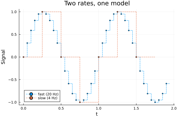
Implementing generic discrete-time components
Discrete-time components can be implemented without specification of the clock or sample interval. To do this, the SampleTime() function is used, which returns the sample-time interval of the associated periodic clock. Here is an example showing how the DiscreteDerivative component is implemented in Dyad:
component DiscreteDerivative@[input clk extends Discrete]
  u = RealInput@[clk]()
  y = RealOutput@[clk]()
  structural parameter Ts::Real = SampleTime()
  parameter k::Real = 1
  parameter initial_output::Real = 0.0
relations
  initial u@(clk-1) = -(Ts/k*initial_output - u@clk)
  y@clk = k * (u@clk - u@(clk-1)) / Ts
end
In this component, the @[input clk extends Discrete] annotation on the component declaration makes the component clock-agnostic — the clock is inherited from the connection context. The structural parameter Ts defaults to SampleTime(), which resolves to the interval of the periodic clock supplied by that context. A component using SampleTime() requires a clock with a defined sample interval.
In order to make components maximally generic, it is often advisable to avoid including Sampler and ZeroOrderHold at the inputs and outputs of a component, and instead let the user manually insert these components where required. Larger components that model complete sampled-data systems may of course contain such operators internally.
Reading results
Every example on this page runs its model through an analysis and plots the result. Two idioms are worth spelling out. The names below are those of the SampledDataDemo model built at the end of this page.
Referring to variables by name. The analysis result can be plotted directly, but to select individual signals you need the simplified system, which carries the symbolic names:
result = SampledDataDemoAnalysis()
model  = artifacts(result, :SimplifiedSystem)
plot(result; idxs = [model.gain.y, model.plant.x])
For raw numerical access, request the underlying solution object instead:
sol = artifacts(result, :RawSolution)
sol[model.plant.x]        # values
sol.t                     # the integrator's time grid
See Analysis Result Interface and the TransientAnalysis artifacts for the full list of what an analysis returns.
Clocked variables have their own time grid. A clocked variable only has a value at its clock's ticks, which are not the integrator's save points. Indexing sol[x] for a clocked x therefore returns the sequence of sample values, but sol.t is the wrong time vector to pair them with. variable_occurrence_times, from the SynchToolkit package that compiles and runs clocked models, returns the matching times:
using SynchToolkit
tv = variable_occurrence_times(model, sol, model.gain.y)
# Vector of time => value pairs
scatter(first.(tv), last.(tv))
The DiscreteComponents library
The components used throughout these tutorials come from DiscreteComponents:
| Group | Components |
|---|---|
| Clocks and clock plumbing | PeriodicClock, ZeroCrossingClock, SampleTimeSource, LastValue, ClockPropagator |
| Continuous ↔ discrete | Sampler, ZeroOrderHold |
| Delays and primitives | UnitDelay, UnitDifference, NDelay, OnOffDelay, DiscreteIntegrator, DiscreteDerivative, DiscreteSlewRateLimiter |
| Linear systems | DiscreteStateSpace, DiscreteTransferFunction |
| Filters | ExponentialFilter, MovingAverageFilter |
| Controllers | DiscretePIDStandard, DiscretePIDParallel, DiscreteBinaryController, SuperTwistingSMC |
| Sensor imperfections | Quantization, NormalNoise, UniformNoise, SampleWithADEffects |
Troubleshooting clock errors
| Symptom | Cause and fix |
|---|---|
Attempted to combine two independent (output) clocks | Two clocks that the compiler cannot prove are the same ended up in one partition — either two clock sources at different rates, or one signal used directly by two partitions. Route cross-rate signals through a LastValue. |
Attempted to combine explicit clocks <a> and <b> | Two different named clock parameters were required to be the same clock. |
The system is unbalanced, or an error mentioning Hold(...) | A discrete-time partition has no clock source at all. Connect a PeriodicClock to one of its signals. |
Attempted to combine clocked value with continuous-time value | A continuous-time signal reached a clocked equation. See Sampled-Data Systems. |
Known limitations
The synchronous-programming support is under active development. The following affect discrete-time models specifically.
One periodic clock cannot be derived from another. Super-sampling or sub-sampling a clock to produce a related clock is not expressible in Dyad. Declare independent
PeriodicClocks and move signals withLastValue.PeriodicClock.offsetis accepted but not yet functional. Leave it at0.Equations in a clocked partition must be causal, i.e. already solved for the variable being computed. Write
x@clk = (u@clk)^(1/3)rather than(x@clk)^3 = u@clk; acausal equations are supported in continuous-time partitions but not in discrete-time ones.Simultaneous ticks on independent clocks have no defined relative order. If two partitions tick at the same instant and the order matters, make the dependency explicit rather than relying on the schedule.
State machines are not available as a modeling construct in discrete-time partitions.
See also
Sampled-Data Systems — combining a discrete-time model with a continuous-time one
Initializing Discrete-Time Components — the
InitialConditionenum and initialization patternsArray Variables in Clocked Components — array-valued clocked state and connectors
Julia Functions, Side Effects and Hardware — calling Julia from clocked equations
Code Generation and Deployment — turning a discrete-time model into a standalone program
Discretizing Continuous-Time Linear Systems — obtaining difference equations from a continuous-time design
Clocks in the syntax manual — the full grammar of clock annotations
DiscreteComponents — the component reference