DC Motor with PI Controller
In this example, a PI controller is set up for speed control of a DC motor. An equivalent circuit diagram is depicted below.

First, a continuous-time velocity controller will be used, we then change the controller to be implemented in discrete time in Discrete-time controller. Finally, we add an outer position controller in Adding a slower outer position loop.
For the basics of modeling a DC motor in Dyad, see the standard library tutorial.
Modeling and simulation
The electrical part consists of a resistance and inductance. The coupling between the electrical and rotational domain is done via an electro-motive force (EMF) component. The voltage across the EMF is proportional to the angular velocity and the current is proportional to the torque. On the mechanical side, viscous friction in, e.g., a bearing and the inertia of the shaft is modeled.
A PI controller with anti-windup should be used as a speed controller. A simulation is performed to verify the tracking performance of the controller and the disturbance rejection capabilities. Download as a Dyad projectdc_motor_pi.zipOpen in Dyad Studio
"""
DC motor with continuous-time PI speed controller.
A step reference is applied at t=0 and a load disturbance at t=1.3s.
"""
test component ContinuousDCMotorPI
  "Electrical components"
  ground = ElectricalComponents.Analog.Basic.Ground()
  source = ElectricalComponents.Analog.Sources.VoltageSource()
  R1 = ElectricalComponents.Analog.Basic.Resistor(R = 0.5)
  L1 = ElectricalComponents.Analog.Basic.Inductor(L = 4.5e-3)
  emf = ElectricalComponents.Analog.Basic.RotationalEMF(k = 0.5)
  "Mechanical components"
  fixed = RotationalComponents.Components.Fixed()
  inertia = RotationalComponents.Components.Inertia(J = 0.02)
  friction = RotationalComponents.Components.Damper(d = 0.01)
  speed_sensor = RotationalComponents.Sensors.VelocitySensor()
  load = RotationalComponents.Sources.TorqueSource()
  "Signal sources"
  ref = BlockComponents.Sources.Step(height = 1, start_time = 0)
  load_step = BlockComponents.Sources.Step(height = -0.3, start_time = 1.3)
  signal_ff = BlockComponents.Sources.Constant(k = 0)
  "Continuous-time PI controller (the derivative part is structurally removed)"
  pi_controller = BlockComponents.Continuous.LimPID(with_D = false, k = 1.1, Ti = 0.035, y_max = 10)
relations
  initial inertia.w = 0
  initial inertia.phi = 0
  initial L1.i = 0
  # Mechanical connections
  connect(fixed.spline, emf.housing, friction.spline_b)
  connect(emf.rotor, friction.spline_a, inertia.spline_a)
  connect(inertia.spline_b, load.spline)
  connect(inertia.spline_b, speed_sensor.spline)
  connect(load.support, fixed.spline)
  connect(load_step.y, load.tau)
  # Controller connections
  connect(ref.y, pi_controller.u_s)
  connect(speed_sensor.w, pi_controller.u_m)
  connect(signal_ff.y, pi_controller.u_ff)
  connect(pi_controller.y, source.V)
  # Electrical connections
  connect(source.p, R1.p)
  connect(R1.n, L1.p)
  connect(L1.n, emf.p)
  connect(emf.n, source.n, ground.g)
end

analysis ContinuousDCMotorPIAnalysis
  extends TransientAnalysis(stop = 2.0)
  model = ContinuousDCMotorPI()
end
Now we can simulate and plot the results:
using Plots
result = ContinuousDCMotorPIAnalysis()
using DyadInterface
model = artifacts(result, :SimplifiedSystem)
p1 = plot(result; idxs = [model.inertia.w, model.ref.y],
    ylabel = "Angular Vel. [rad/s]",
    labels = ["Measurement" "Reference"],
    title = "DC Motor with Speed Controller")
p2 = plot(result; idxs = model.load_step.y, ylabel = "Disturbance [Nm]", label = "")
plot(p1, p2, layout = (2, 1))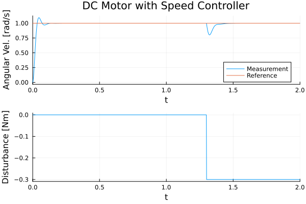
Discrete-time controller
Until now, we have modeled both the physical part of the system, the DC motor, and the control system, in continuous time. In practice, it is common to implement control systems on a computer operating at a fixed sample rate, i.e., in discrete time. A system containing both continuous-time parts and discrete-time parts is often referred to as a "sampled-data system". The DiscreteComponents library contains several components to model such systems. See also the Discrete-Time Modeling tutorial.
Below, we re-model the system, this time with a discrete-time controller: DiscretePIDStandard. To interface between the continuous and discrete parts of the model, we make use of a Sampler (driven by a PeriodicClock) and a ZeroOrderHold component. Apart from these components, the model is the same as before.
"""
DC motor with discrete-time PI speed controller.
A Sampler driven by a PeriodicClock samples the speed at 200 Hz, and a
ZeroOrderHold converts the discrete controller output back to continuous time.
"""
test component DiscreteDCMotorPI
  "Electrical components"
  ground = ElectricalComponents.Analog.Basic.Ground()
  source = ElectricalComponents.Analog.Sources.VoltageSource()
  R1 = ElectricalComponents.Analog.Basic.Resistor(R = 0.5)
  L1 = ElectricalComponents.Analog.Basic.Inductor(L = 4.5e-3)
  emf = ElectricalComponents.Analog.Basic.RotationalEMF(k = 0.5)
  "Mechanical components"
  fixed = RotationalComponents.Components.Fixed()
  inertia = RotationalComponents.Components.Inertia(J = 0.02)
  friction = RotationalComponents.Components.Damper(d = 0.01)
  speed_sensor = RotationalComponents.Sensors.VelocitySensor()
  angle_sensor = RotationalComponents.Sensors.AngleSensor()
  load = RotationalComponents.Sources.TorqueSource()
  "Signal sources"
  ref = BlockComponents.Sources.Step(height = 1, start_time = 0)
  load_step = BlockComponents.Sources.Step(height = -0.3, start_time = 1.3)
  "Discrete-time components"
  sampler = DiscreteComponents.Sampler()
  "The continuous reference must be sampled before entering the discrete partition"
  ref_sampler = DiscreteComponents.Sampler()
  clock = DiscreteComponents.PeriodicClock(dt = 0.005)
  pi_controller = DiscreteComponents.DiscretePIDStandard(K = 1, Ti = 0.035, y_max = 10, with_D = false)
  zoh = DiscreteComponents.ZeroOrderHold()
relations
  initial inertia.w = 0
  initial inertia.phi = 0
  initial L1.i = 0
  # Mechanical connections
  connect(fixed.spline, emf.housing, friction.spline_b)
  connect(emf.rotor, friction.spline_a, inertia.spline_a)
  connect(inertia.spline_b, load.spline)
  connect(inertia.spline_b, speed_sensor.spline, angle_sensor.spline)
  connect(load.support, fixed.spline)
  connect(load_step.y, load.tau)
  # Controller connections
  connect(ref.y, ref_sampler.u)
  connect(ref_sampler.y, pi_controller.u_s)
  connect(speed_sensor.w, sampler.u)
  connect(sampler.y, pi_controller.u_m, clock.y)
  connect(pi_controller.y, zoh.u)
  connect(zoh.y, source.V)
  # Electrical connections
  connect(source.p, R1.p)
  connect(R1.n, L1.p)
  connect(L1.n, emf.p)
  connect(emf.n, source.n, ground.g)
end

analysis DiscreteDCMotorPIAnalysis
  extends TransientAnalysis(stop = 2.0)
  model = DiscreteDCMotorPI()
enddisc_result = DiscreteDCMotorPIAnalysis()
disc_model = artifacts(disc_result, :SimplifiedSystem)
cont_model = artifacts(result, :SimplifiedSystem)
plot(result; idxs = cont_model.inertia.w, ylabel = "Angular Vel. [rad/s]",
label = "Measurement (cont. controller)", title = "DC Motor with Speed Controller")
plot!(disc_result; idxs = disc_model.inertia.w,
label = "Measurement (disc. controller)", legend = :bottomleft)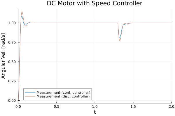
In the plot above, we compare the result of the discrete-time control system to the continuous-time result from before. We see that with the chosen sample interval of dt = 0.005 (provided to the PeriodicClock), we have a slight degradation in the control performance as a consequence of the discretization.
Adding a slower outer position loop
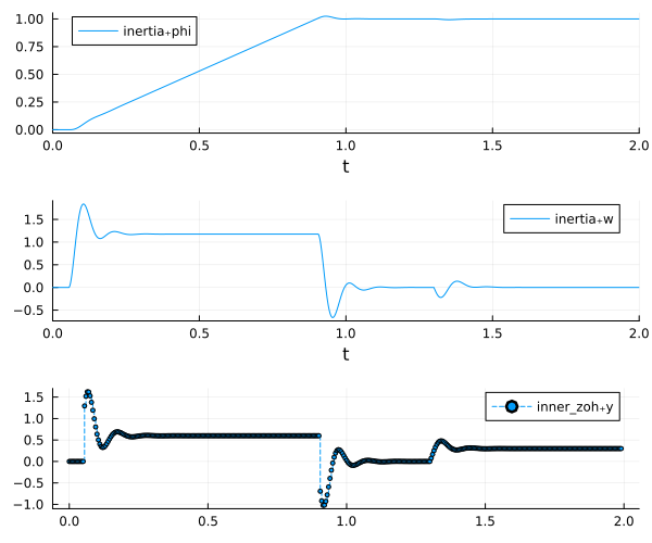
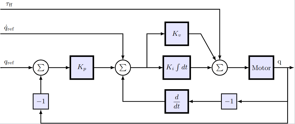
Below, we add an outer control loop that controls the position of the motor by manipulating the reference to the inner speed controller. This is a common control strategy, often referred to as cascade control.
"""
Cascade position-speed control of a DC motor.
An outer proportional position controller provides the speed reference
for the inner discrete-time PI speed controller. The position reference
is differentiated to provide a feedforward velocity term.
"""
test component CascadeDCMotorPI
  # Inner speed control loop (same as DiscreteDCMotorPI but without external ref)
  "Electrical components"
  ground = ElectricalComponents.Analog.Basic.Ground()
  source = ElectricalComponents.Analog.Sources.VoltageSource()
  R1 = ElectricalComponents.Analog.Basic.Resistor(R = 0.5)
  L1 = ElectricalComponents.Analog.Basic.Inductor(L = 4.5e-3)
  emf = ElectricalComponents.Analog.Basic.RotationalEMF(k = 0.5)
  "Mechanical components"
  fixed = RotationalComponents.Components.Fixed()
  inertia = RotationalComponents.Components.Inertia(J = 0.02)
  friction = RotationalComponents.Components.Damper(d = 0.01)
  speed_sensor = RotationalComponents.Sensors.VelocitySensor()
  angle_sensor = RotationalComponents.Sensors.AngleSensor()
  load = RotationalComponents.Sources.TorqueSource()
  load_step = BlockComponents.Sources.Step(height = -0.3, start_time = 1.3)
  "Inner discrete-time speed controller"
  inner_sampler = DiscreteComponents.Sampler()
  inner_clock = DiscreteComponents.PeriodicClock(dt = 0.005)
  inner_pi = DiscreteComponents.DiscretePIDStandard(K = 1, Ti = 0.035, y_max = 10, with_D = false)
  inner_zoh = DiscreteComponents.ZeroOrderHold()
  "Outer position controller"
  ref = BlockComponents.Sources.Ramp(height = 1, start_time = 0.05, duration = 0.85)
  "The continuous reference must be sampled before entering the discrete partition"
  ref_sampler = DiscreteComponents.Sampler()
  outer_sampler = DiscreteComponents.Sampler()
  outer_clock = DiscreteComponents.PeriodicClock(dt = 0.005)
  p_controller = DiscreteComponents.DiscretePIDStandard(K = 20, with_D = false, with_I = false)
  ref_diff = DiscreteComponents.DiscreteDerivative()
  add = BlockComponents.Math.Add()
  gain = BlockComponents.Math.Gain(k = 1)
relations
  initial inertia.w = 0
  initial inertia.phi = 0
  initial L1.i = 0
  # Mechanical connections
  connect(fixed.spline, emf.housing, friction.spline_b)
  connect(emf.rotor, friction.spline_a, inertia.spline_a)
  connect(inertia.spline_b, load.spline)
  connect(inertia.spline_b, speed_sensor.spline, angle_sensor.spline)
  connect(load.support, fixed.spline)
  connect(load_step.y, load.tau)
  # Inner speed controller
  connect(speed_sensor.w, inner_sampler.u)
  connect(inner_sampler.y, inner_pi.u_m, inner_clock.y)
  connect(inner_pi.y, inner_zoh.u)
  connect(inner_zoh.y, source.V)
  # Outer position controller
  connect(ref.y, ref_sampler.u)
  connect(ref_sampler.y, p_controller.u_s, ref_diff.u)
  connect(ref_diff.y, add.u1)
  connect(p_controller.y, add.u2)
  connect(add.y, gain.u)
  connect(gain.y, inner_pi.u_s)
  connect(angle_sensor.phi, outer_sampler.u)
  connect(outer_sampler.y, p_controller.u_m, outer_clock.y)
  # Electrical connections
  connect(source.p, R1.p)
  connect(R1.n, L1.p)
  connect(L1.n, emf.p)
  connect(emf.n, source.n, ground.g)
end

analysis CascadeDCMotorPIAnalysis
  extends TransientAnalysis(stop = 2.0)
  model = CascadeDCMotorPI()
endcascade_result = CascadeDCMotorPIAnalysis()
cascade_model = artifacts(cascade_result, :SimplifiedSystem)
plot(cascade_result; idxs = [cascade_model.inertia.phi, cascade_model.inertia.w, cascade_model.inner_zoh.y],
layout = (3, 1), size = (600, 500))