
Discretizing Continuous-Time Linear Systems
Control design is often done in continuous time, but a controller that runs on a computer is running in discrete time. This page covers converting between the two with ControlSystems.jl and making use of the result in a clocked Dyad model.
See Discrete-Time Modeling for clocks, and Array Variables in Clocked Components for the discrete linear-system components.
c2d and the choice of method
c2d(sys, Ts, method) converts a continuous-time system to a periodic discrete-time system at sample interval Ts. d2c converts in the other direction. The discretization methods differ in what they preserve:
| Method | Preserves | Use when |
|---|---|---|
:zoh | The response to a piecewise-constant input, exactly. State components keep their meaning. | Often used when discretizing a plant model driven through a zero-order hold. |
:foh | The response to a piecewise-linear input. State meaning preserved. | The input is better modelled as ramping between samples. |
:tustin | The frequency response, approximately, with no aliasing of the imaginary axis. Changes the state basis. | Commonly used when discretizing a controller. |
:fwdeuler | Nothing in particular; simplest possible. | Quick approximations at sample rates far above the dynamics. Generally not recommended. |
:tustin (the bilinear transform) accepts w_prewarp, which makes the discrete-time and continuous-time frequency responses agree exactly at that frequency instead of only at DC — useful when a specific crossover or notch frequency matters.
A rule of thumb is: ZoH for plant models, Tustin for controllers. ZoH matches what the hardware actually does to a plant input, while Tustin gives the controller the frequency-domain behaviour it was designed for.
Getting the coefficients into a Dyad component
DiscreteTransferFunction takes numerator and denominator coefficient arrays, and they are exactly what ControlSystems.jl's numvec/denvec return — descending powers of
Discretizing a PI controller
using ControlSystemsBase

Ts = 0.05
K, Ti = 2.0, 0.5
C  = K * (1 + tf(1.0, [Ti, 0.0]))
Cz = c2d(ss(C), Ts, :tustin)

b = numvec(tf(Cz))[1]
a = denvec(tf(Cz))[1]
(b, a)
([2.1, -1.9000000000000001], [1.0, -1.0])Those two vectors go straight into the component. The plant is discretized with ZoH for comparison:
P  = ss(tf(1.0, [0.5, 1.0]))
Pz = c2d(P, Ts, :zoh)
(numvec(tf(Pz))[1], denvec(tf(Pz))[1])
([0.09516258196404037], [1.0, -0.9048374180359594])A closed loop built from discretized designs
Both blocks below carry the coefficients computed above. Download as a Dyad projectc2d.zipOpen in Dyad Studio
"""
Discrete-time PI controller (Tustin) driving a discrete-time plant (ZoH), with the
coefficients taken from `c2d`. Both blocks run on the same 20 Hz clock.
"""
test component DiscretizedLoop
  ref = BlockComponents.Sources.Step(height = 1.0, start_time = 0.1)
  ref_sampler = DiscreteComponents.Sampler()
  clock = DiscreteComponents.PeriodicClock(dt = 0.05)
  err = BlockComponents.Math.Add(k2 = -1)
  "PI controller, c2d(..., :tustin)"
  ctrl = DiscreteComponents.DiscreteTransferFunction(b = [2.1, -1.9], a = [1.0, -1.0])
  "Plant, c2d(..., :zoh)"
  plant = DiscreteComponents.DiscreteTransferFunction(
      b = [0.09516258196404037], a = [1.0, -0.9048374180359594])
relations
  connect(ref.y, ref_sampler.u)
  connect(ref_sampler.y, clock.y, err.u1)
  connect(err.y, ctrl.u)
  connect(ctrl.y, plant.u)
  connect(plant.y, err.u2)
end

analysis DiscretizedLoopAnalysis
  extends TransientAnalysis(stop = 2.0)
  model = DiscretizedLoop()
endusing Plots
using DyadInterface
result = DiscretizedLoopAnalysis()
model = artifacts(result, :SimplifiedSystem)
p1 = plot(result; idxs = model.plant.y, title = "Plant output")
p2 = plot(result; idxs = model.ctrl.y, title = "Control signal")
plot(p1, p2; layout = (2, 1), legend = false, xlabel = "t",
size = (600, 430), plot_title = "Loop assembled from c2d designs")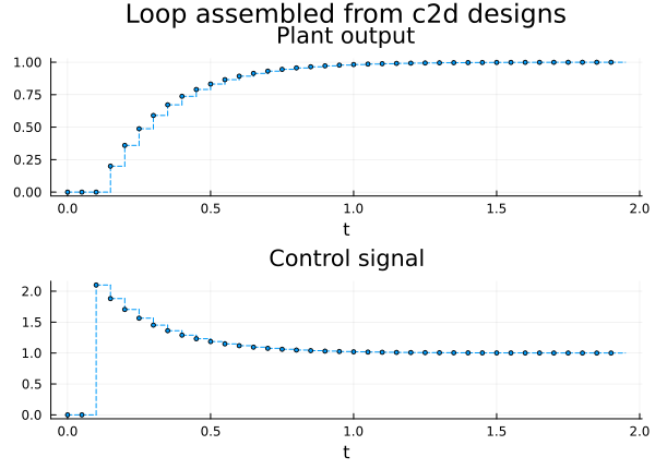
The same loop can be evaluated in Julia before it is ever built in Dyad, which is the quickest way to check that a discretization did what you expected:
Lz = Cz * Pz
Tz = feedback(Lz)
res = step(Tz, 2.0)
plot(res.t, vec(res.y); seriestype = :steppost, legend = false,
     xlabel = "t", title = "Same loop, evaluated with ControlSystems.jl")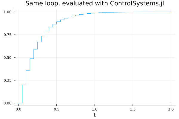
Discretization inside components
Some components do their own discretization rather than taking coefficients. The integrating and differentiating blocks take a DiscretizationMethod:
Forward()— forward Euler,Backward()— backward Euler,Trapezoidal()—c2d(..., :tustin)
DiscreteIntegrator takes method, and the discrete-time PID blocks take Imethod and Dmethod separately, a discrete-time PID controller commonly uses forward Euler on the integral term and backward Euler on the derivative term.
Choosing Trapezoidal there is equivalent to designing the term in continuous time and applying c2d(..., :tustin) to it.
Discretizing noise covariance
When a state estimator is discretized, the process-noise covariance has to be converted too — carrying a continuous-time Qc straight into a discrete filter gives the wrong noise level, and the error depends on Ts. c2d has methods for this:
Qd     = c2d(sys::StateSpace{Continuous}, Qc, Ts)
Qd, Rd = c2d(sys::StateSpace{Discrete}, Qc, Rc; opt = :c)
See the c2d documentation for the assumptions behind each form, in particular how a rank-deficient Qc is handled.
Several DyadControlSystems analyses discretize the plant internally and expose the sample interval as an argument, so you do not always have to do this yourself — see Pole placement, LQG analysis and State estimation.
See also
Discrete-Time Modeling — clocks, partitions and reading results
Sampled-Data Systems — combining discrete-time and continuous-time models
Array Variables in Clocked Components —
DiscreteTransferFunctionandDiscreteStateSpaceFrequency-response analysis — measuring the loop you built
ControlSystems.jl: Analysis of sampled-data systems — how ZoH interacts with continuous-time analysis
ControlSystems.jl: Performance considerations — numerical caveats when discretizing
RobustAndOptimalControl.jl and DyadControlSystems — the design side