TUTORIAL

Initializing Discrete-Time Components

A discrete-time component computes each sample from earlier samples, so before the first tick it needs values for those earlier samples, provided as initial conditions. This page covers how to supply them, and the convention the DiscreteComponents library uses to let a user of a component choose how it starts up.

See Discrete-Time Modeling for clocks and the shift operators, and Clocks for the syntax reference.

Initial conditions refer to the past

The initial condition of a clocked variable is given with initial and a past clock reference:

initial x@(clk-1) = 1.0

The shift is there because the update performed at the first tick,   , reads  . Setting x@clk instead would fix the result of the first update rather than the state it starts from.

One initial equation is needed for every shift depth the component reads. A component that uses x@(clk-2) needs both:

initial x@(clk-1) = 0.0
initial x@(clk-2) = 0.0

When the depth is itself a parameter, generate the equations with a loop. This is how NDelay fills its delay line:

component NDelay@[input clk extends Discrete]
  u = RealInput@[clk]() {^u}
  y = RealOutput@[clk]() {^y}
  structural parameter n::Integer
  parameter initial_condition::Real = 0
relations
  y = u@(clk-n)
  for i in 1:n
    initial u@(clk-i) = initial_condition
  end
end

To set the initial condition of a subcomponent's variable from a parent, write the equation in the parent's relations block — for example initial secondorder.x = 0.0.

The InitialCondition enum

A raw initial x@(clk-1) = … fixes the component's internal state, which is rarely what a user of the component wants to think about. They usually want to say "start with your output at 5.0", or "start in steady state". The DiscreteComponents.InitialCondition enum expresses that intent:

Variant	Meaning
InitialOutput(y0)	The first emitted output should equal y0.
InitialState(x0)	The internal state starts at x0.
SteadyState	Start in equilibrium for the current input, so the output does not jump at .
InitialOutputArray(y0)	InitialOutput for a vector-valued output.
InitialStateArray(x0)	InitialState for a vector-valued state.

Not every variant makes sense for every component, and each component documents which ones it accepts.

Passing one when instantiating a component looks like this:

filt = DiscreteComponents.ExponentialFilter(a = 0.2,
         initialization = DiscreteComponents.InitialCondition.InitialOutput(y0 = -1))

The Sliding-Mode Control example uses exactly this to start its filter and its derivative block at known values.

Implementing the enum in your own component

The component declares a structural parameter of the enum type and switches on it in relations. Each case supplies whatever initial equations that mode implies. (See Enums and switch-case for the general construct.)

Here is ExponentialFilter, which is the smallest complete illustration:

component ExponentialFilter@[input clk extends Discrete]
  u = RealInput@[clk]() {^u}
  y = RealOutput@[clk]() {^y}
  parameter a::Real = 0.1
  structural parameter initialization::InitialCondition = DiscreteComponents.InitialCondition.InitialOutput(y0=0.0)
relations
  y@clk = (1 - a) * y@(clk-1) + a * u@clk

  switch initialization
  case InitialOutput
    initial y@(clk-1) = (initialization.y0 - a*u@clk) / (1 - a)
  case SteadyState
    initial y@(clk-1) = u@clk
  case InitialState
    initial y@(clk-1) = initialization.x0
  end
end

Three patterns matter here. The first is visible in the listing above; the other two are shown with the components that need them.

Solve backwards through the update equation

The InitialOutput case is not initial y@(clk-1) = initialization.y0. The value being set is the state before the first update, and the first update will transform it. To make the first emitted sample equal y0, invert the update equation. For the filter,       gives

which is exactly the expression in the listing. Writing the naive version instead would leave the first output off by one filter step.

InitialState, by contrast, does assign directly — that is what distinguishes the two modes.

Reject the modes you do not support

Some modes are meaningless for some components — a pure integrator has no steady state for a non-zero input, and a scalar block cannot use an array variant. Put error(...) on the right-hand side of the initial equation for those cases, so the user gets a clear message instead of a confusing numerical result:

  switch initialization
  case InitialOutput
    initial x@(clk-1) = initialization.y0
  case InitialState
    initial x@(clk-1) = initialization.x0
  case SteadyState
    initial x@(clk-1) = error("SteadyState is not supported for this component; use InitialOutput or InitialState")
  end

Switches can nest

When a component has two structural choices that interact, nest the switches. The DiscreteIntegrator picks a discretization method and an initialization mode, and the back-solved expression differs per method — forward Euler reads u@(clk-1) while backward Euler reads u@clk, so the correction term is not the same:

  switch method
  case Forward
    initial u@(clk-1) = 0
    x@clk = x@(clk-1) + k * Ts * u@(clk-1)
    switch initialization
    case InitialOutput
      initial x@(clk-1) = initialization.y0
    ...
    end
  case Backward
    x@clk = x@(clk-1) + k * Ts * u@clk
    switch initialization
    case InitialOutput
      initial x@(clk-1) = initialization.y0 - k*Ts*u@clk
    ...
    end
  end

A worked example

Below, three exponential filters see the same constant input of 1.0 but start differently: one with its first output forced to 2.0, one with its internal state set to -1.0, and one in steady state. All three converge to the input; only their transients differ. Download as a Dyad projectdiscreteinit.zipOpen in Dyad Studio›

"""
Three identically-parameterized exponential filters started three different ways,
to show what each `InitialCondition` variant does to the first samples.
"""
test component InitializationDemo
  source = BlockComponents.Sources.Constant(k = 1.0)
  sampler = DiscreteComponents.Sampler()
  clock = DiscreteComponents.PeriodicClock(dt = 0.1)
  "First output forced to 2.0"
  filt_out = DiscreteComponents.ExponentialFilter(a = 0.2,
      initialization = DiscreteComponents.InitialCondition.InitialOutput(y0 = 2.0))
  "Internal state forced to -1.0"
  filt_state = DiscreteComponents.ExponentialFilter(a = 0.2,
      initialization = DiscreteComponents.InitialCondition.InitialState(x0 = -1.0))
  "Started in equilibrium with the input"
  filt_ss = DiscreteComponents.ExponentialFilter(a = 0.2,
      initialization = DiscreteComponents.InitialCondition.SteadyState())
relations
  connect(source.y, sampler.u)
  connect(sampler.y, clock.y, filt_out.u, filt_state.u, filt_ss.u)
end

analysis InitializationDemoAnalysis
  extends TransientAnalysis(stop = 2.0)
  model = InitializationDemo()
end

using Plots
using DyadInterface
result = InitializationDemoAnalysis()
model = artifacts(result, :SimplifiedSystem)
p1 = plot(result; idxs = model.filt_out.y, title = "InitialOutput(y0 = 2.0)")
p2 = plot(result; idxs = model.filt_state.y, title = "InitialState(x0 = -1.0)")
p3 = plot(result; idxs = model.filt_ss.y, title = "SteadyState")
plot(p1, p2, p3; layout = (3, 1), legend = false, xlabel = "t", ylabel = "y",
     size = (600, 550), plot_title = "Same filter, three initializations")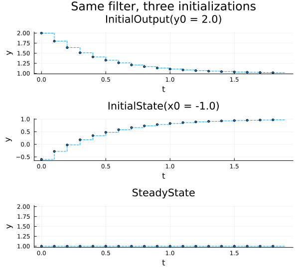

The SteadyState panel is flat at the input value: the filter starts already in equilibrium, so it never moves. The InitialOutput panel begins at exactly 2.0 — that is the guarantee the back-solved initial state buys — and decays towards the input from above. The InitialState panel starts at -0.6, not at -1.0: setting the stored state means the first output is already one filter step away from it,     . It approaches the input from below.

Limitations

• You cannot ask for an output and have the state inferred for you. Writing y@clk = y0 does not cause y@(clk-1) to be back-solved. The component author has to do the inversion, which is why the InitialOutput cases above look the way they do. This limitation exists due to the lack of a general nonlinear solver for initialization of discrete-time partitions (which in general would have an unbounded execution time).

• Only explicit initial equations are supported. initial modifiers on variables are not yet supported for clocked variables, use initial equations instead.

See also

• Discrete-Time Modeling — clocks, shift operators and partitions

• Array Variables in Clocked Components — the array initialization variants

• Clocks — syntax reference for clock annotations and initial

• Enums and switch-case — the general enum construct

• Sliding-Mode Control — a model that sets initial conditions on two blocks

• DiscreteComponents — per-component documentation of the accepted modes