
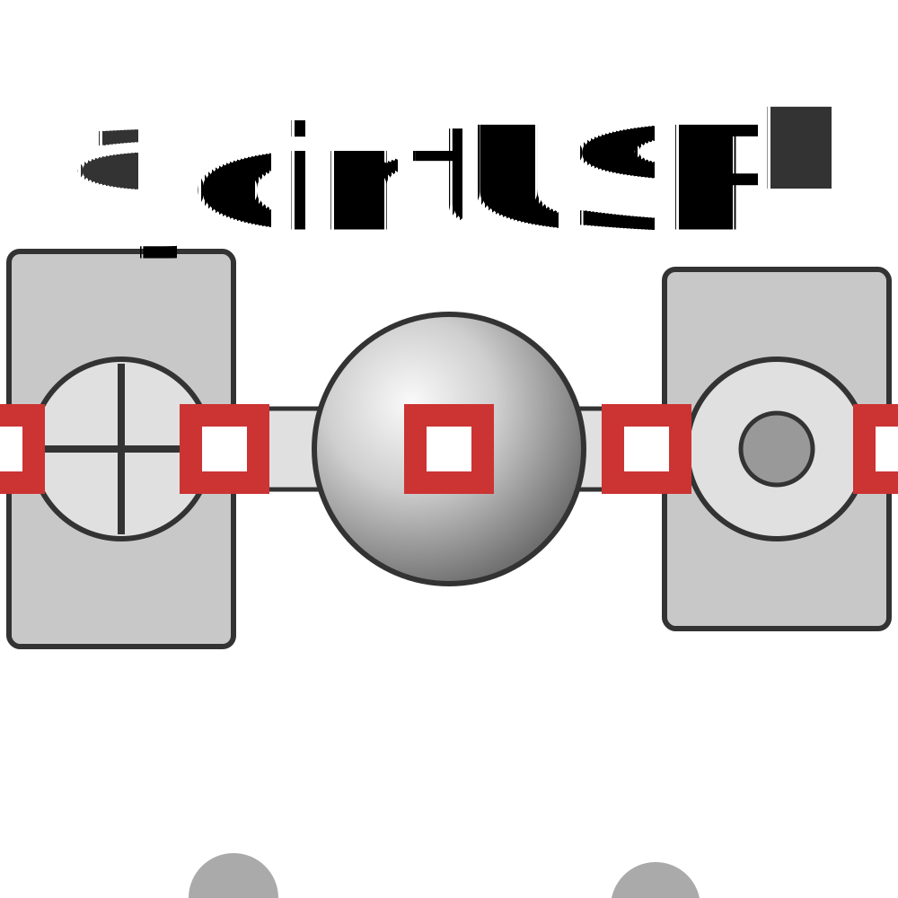
JointUSR
Joint assembly consisting of a universal joint at frame_a, a spherical joint in the middle, and a revolute joint at frame_b (hence USR). The universal and spherical joints are connected by rod1 (a UniversalSpherical assembly), and the spherical and revolute joints by rod2 (a FixedTranslation).
The assembly has no mass and no inertia and introduces neither constraints nor potential states: the non-linear loop closure is solved analytically. Use it in kinematic loops whenever possible, since it is far more efficient than the equivalent loop built from basic joints plus a cut joint.
There is a singularity when n1_a is parallel to the rod direction rRod1_ia. Choose n1_a orthogonal to rRod1_ia in the initial configuration when possible. Two configurations satisfy the constraints; which one the mechanism is assembled in is selected automatically at initialization as the one closest to phi_guess. Set positive_branch to force a branch instead.
This component extends from PartialTwoFrames
Usage
MultibodyComponents.JointUSR(n1_a=[0, 0, 1], n_b=[0, 0, 1], rRod1_ia=[1, 0, 0], rRod2_ib=[-1, 0, 0], phi_offset=0, phi_guess=0, rod_radius=0.05, rod_color=[0.5, 0, 0.5, 1], rod1_length=norm_(rRod1_ia), e_b=n_b / norm_(n_b))
Parameters:
| Name | Description | Units | Default value |
|---|---|---|---|
positive_branch | Force a branch of the analytic loop-closure solution instead of selecting it automatically from the guess value | – | missing |
n_b_nonzero | Structural sparsity mask for the frame_b revolute axis (passed to the analytic revolute). | – | [true, true, true] |
n1_a | Axis 1 of the universal joint, resolved in frame_a | – | [0, 0, 1] |
n_b | Axis of the revolute joint, resolved in frame_b | – | [0, 0, 1] |
rRod1_ia | Vector from frame_a origin to the spherical joint, resolved in frame_ia | – | [1, 0, 0] |
rRod2_ib | Vector from frame_ib origin to the spherical joint, resolved in frame_ib | – | [-1, 0, 0] |
phi_offset | Relative angle offset of the revolute joint | – | 0 |
phi_guess | Guess value for the revolute angle at the initial time | – | 0 |
rod_radius | Rendering radius of the rods | – | 0.05 |
rod_color | RGBA color of the rods | – | [0.5, 0, 0.5, 1] |
Connectors
frame_a- Frame3D is the fundamental 3D connector used for 6DOF motion. Most components have one or severalFrame
connectors that can be connected together (Frame3D)
frame_b- Frame3D is the fundamental 3D connector used for 6DOF motion. Most components have one or severalFrame
connectors that can be connected together (Frame3D)
frame_ia- Frame3D is the fundamental 3D connector used for 6DOF motion. Most components have one or severalFrame
connectors that can be connected together (Frame3D)
frame_ib- Frame3D is the fundamental 3D connector used for 6DOF motion. Most components have one or severalFrame
connectors that can be connected together (Frame3D)
frame_im- Frame3D is the fundamental 3D connector used for 6DOF motion. Most components have one or severalFrame
connectors that can be connected together (Frame3D)
axis- This connector represents a rotational spline with angle and torque as the potential and flow variables, respectively. (Spline)bearing- This connector represents a rotational spline with angle and torque as the potential and flow variables, respectively. (Spline)
Variables
| Name | Description | Units |
|---|---|---|
aux | Denominator used to compute the rod force | – |
f_rod | Constraint force in the direction of rod1 (positive if the rod is pressed) | – |
Behavior
Source
"""
Joint assembly consisting of a **universal** joint at `frame_a`, a
**spherical** joint in the middle, and a **revolute** joint at `frame_b`
(hence USR). The universal and spherical joints are connected by `rod1`
(a `UniversalSpherical` assembly), and the spherical and revolute joints by
`rod2` (a `FixedTranslation`).

The assembly has no mass and no inertia and introduces neither constraints nor
potential states: the non-linear loop closure is solved analytically. Use it in
kinematic loops whenever possible, since it is far more efficient than the
equivalent loop built from basic joints plus a cut joint.

There is a singularity when `n1_a` is parallel to the rod direction `rRod1_ia`.
Choose `n1_a` orthogonal to `rRod1_ia` in the initial configuration when
possible. Two configurations satisfy the constraints; which one the mechanism is
assembled in is selected automatically at initialization as the one closest to
`phi_guess`. Set `positive_branch` to force a branch instead.
"""
component JointUSR
  extends PartialTwoFrames()
  "Frame fixed in rod1 at the origin of frame_a"
  frame_ia = Frame3D() {
    "Dyad": {
      "placement": {
        "diagram": {"iconName": "default", "x1": 200, "y1": 450, "x2": 300, "y2": 550, "rot": 0}
      },
      "tags": []
    }
  }
  "Frame fixed in rod2 at the revolute side (= rod2.frame_a)"
  frame_ib = Frame3D() {
    "Dyad": {
      "placement": {
        "diagram": {"iconName": "default", "x1": 670, "y1": 450, "x2": 770, "y2": 550, "rot": 0}
      },
      "tags": []
    }
  }
  "Frame fixed in rod2 at the spherical side (= rod2.frame_b)"
  frame_im = Frame3D() {
    "Dyad": {
      "placement": {
        "diagram": {"iconName": "default", "x1": 450, "y1": 450, "x2": 550, "y2": 550, "rot": 0}
      },
      "tags": []
    }
  }
  "Rotational flange driving the revolute joint"
  axis = Spline() {
    "Dyad": {
      "placement": {
        "diagram": {"iconName": "default", "x1": 680, "y1": 960, "x2": 780, "y2": 1060, "rot": 0}
      },
      "tags": []
    }
  }
  "Rotational flange of the revolute joint bearing"
  bearing = Spline() {
    "Dyad": {
      "placement": {
        "diagram": {"iconName": "default", "x1": 210, "y1": 950, "x2": 310, "y2": 1050, "rot": 0}
      },
      "tags": []
    }
  }
  rod1 = UniversalSpherical(n1_a = n1_a, rRod_ia = rRod1_ia, kinematic_constraint = false, constraint_residue_external = true, rod_radius = rod_radius, color = rod_color, sphere_color = [0, 0, 0, 0]) {
    "Dyad": {
      "placement": {
        "diagram": {"iconName": "default", "x1": 300, "y1": 560, "x2": 400, "y2": 660, "rot": 0}
      },
      "tags": []
    }
  }
  rod2 = FixedTranslation(r = rRod2_ib, radius = rod_radius, color = rod_color) {
    "Dyad": {
      "placement": {
        "diagram": {"iconName": "default", "x1": 660, "y1": 450, "x2": 560, "y2": 550, "rot": 0}
      },
      "tags": []
    }
  }
  revolute = RevoluteWithLengthConstraint(n = n_b, n_nonzero = n_b_nonzero, length_constraint = rod1_length, phi_offset = phi_offset, phi_guess = phi_guess, positive_branch = positive_branch) {
    "Dyad": {
      "placement": {
        "diagram": {"iconName": "default", "x1": 790, "y1": 680, "x2": 690, "y2": 780, "rot": 0}
      },
      "tags": []
    }
  }
  "Force a branch of the analytic loop-closure solution instead of selecting it automatically from the guess value"
  structural parameter positive_branch::Boolean = missing
  "Axis 1 of the universal joint, resolved in frame_a"
  parameter n1_a::Real[3] = [0, 0, 1]
  "Axis of the revolute joint, resolved in frame_b"
  parameter n_b::Real[3] = [0, 0, 1]
  "Structural sparsity mask for the frame_b revolute axis (passed to the analytic revolute)."
  structural parameter n_b_nonzero::Boolean[3] = [true, true, true]
  "Vector from frame_a origin to the spherical joint, resolved in frame_ia"
  parameter rRod1_ia::Real[3] = [1, 0, 0]
  "Vector from frame_ib origin to the spherical joint, resolved in frame_ib"
  parameter rRod2_ib::Real[3] = [-1, 0, 0]
  "Relative angle offset of the revolute joint"
  parameter phi_offset::Real = 0
  "Guess value for the revolute angle at the initial time"
  parameter phi_guess::Real = 0
  "Rendering radius of the rods"
  parameter rod_radius::Real = 0.05
  "RGBA color of the rods"
  parameter rod_color::Real[4] = [0.5, 0, 0.5, 1]
  final parameter rod1_length::Real = norm_(rRod1_ia)
  final parameter e_b::Real[3] = n_b / norm_(n_b)
  "Denominator used to compute the rod force"
  variable aux::Real
  "Constraint force in the direction of rod1 (positive if the rod is pressed)"
  variable f_rod::Real
relations
  aux = dot(cross(e_b, rRod2_ib), resolve_relative(rod1.eRod_a, rod1.frame_a.R, rod1.frame_b.R))
  # The guard against division by zero must preserve the sign of aux (MSL:
  # `noEvent(if abs(aux) < 1e-10 then 1e-10 else aux)`); flattening it to
  # max(abs(aux), 1e-10) flips the sign of f_rod whenever aux < 0 (e.g. for
  # mirrored suspension assemblies), making the analytic force distribution
  # inconsistent with the torque balance.
  f_rod = (-revolute.tau - dot(e_b, frame_ib.tau + frame_im.tau + cross(rRod2_ib, frame_im.f) - cross(rRod2_ib, resolve_relative(rod1.f_b_a1, rod1.frame_a.R, rod1.frame_b.R)))) / ifelse(abs(aux) < 1e-10, 1e-10, aux)
  rod1.constraint_residue = rod1.f_rod - f_rod
  revolute.r_a = resolve2(frame_b.R, frame_a.r_0 - frame_b.r_0)
  revolute.r_b = rRod2_ib
  connect(revolute.frame_a, frame_b) {
    "Dyad": {
      "edges": [{"S": 1, "M": [{"x": 850, "y": 730}, {"x": 850, "y": 500}], "E": 2}],
      "renderStyle": "standard"
    }
  }
  connect(rod2.frame_a, frame_ib) {"Dyad": {"edges": [{"S": 1, "M": [], "E": 2}], "renderStyle": "standard"}}
  connect(rod1.frame_ia, frame_ia) {
    "Dyad": {
      "edges": [{"S": 1, "M": [{"x": 345, "y": 500}], "E": 2}],
      "renderStyle": "standard"
    }
  }
  connect(rod2.frame_b, frame_im) {"Dyad": {"edges": [{"S": 1, "M": [], "E": 2}], "renderStyle": "standard"}}
  connect(rod1.frame_a, frame_a) {
    "Dyad": {
      "renderStyle": "standard",
      "edges": [{"S": 1, "M": [{"x": 0, "y": 610}], "E": 2}]
    }
  }
  connect(revolute.frame_b, frame_ib) {
    "Dyad": {
      "edges": [{"S": 1, "M": [{"x": 690, "y": 540}, {"x": 720, "y": 540}], "E": 2}],
      "renderStyle": "standard"
    }
  }
  connect(rod1.frame_b, frame_im) {
    "Dyad": {
      "edges": [{"S": 1, "M": [{"x": 500, "y": 610}], "E": 2}],
      "renderStyle": "standard"
    }
  }
  connect(bearing, revolute.bearing) {
    "Dyad": {
      "edges": [
        {
          "S": 1,
          "M": [{"x": 300, "y": 1000}, {"x": 300, "y": 880}, {"x": 762, "y": 880}],
          "E": 2
        }
      ],
      "renderStyle": "standard"
    }
  }
  connect(revolute.axis, axis) {
    "Dyad": {
      "renderStyle": "standard",
      "edges": [{"S": 1, "M": [{"x": 720, "y": 1010}], "E": 2}]
    }
  }
metadata {
  "Dyad": {
    "icons": {"default": "dyad://MultibodyComponents/JointUSR.svg"},
    "labels": [
      {
        "label": "$(instance)",
        "x": 500,
        "y": 200,
        "rot": 0,
        "attrs": {"font-size": "160"}
      }
    ]
  }
}
end
Flattened Source
"""
Joint assembly consisting of a **universal** joint at `frame_a`, a
**spherical** joint in the middle, and a **revolute** joint at `frame_b`
(hence USR). The universal and spherical joints are connected by `rod1`
(a `UniversalSpherical` assembly), and the spherical and revolute joints by
`rod2` (a `FixedTranslation`).

The assembly has no mass and no inertia and introduces neither constraints nor
potential states: the non-linear loop closure is solved analytically. Use it in
kinematic loops whenever possible, since it is far more efficient than the
equivalent loop built from basic joints plus a cut joint.

There is a singularity when `n1_a` is parallel to the rod direction `rRod1_ia`.
Choose `n1_a` orthogonal to `rRod1_ia` in the initial configuration when
possible. Two configurations satisfy the constraints; which one the mechanism is
assembled in is selected automatically at initialization as the one closest to
`phi_guess`. Set `positive_branch` to force a branch instead.
"""
component JointUSR
  frame_a = Frame3D() {
    "Dyad": {
      "placement": {
        "diagram": {"iconName": "default", "x1": -50, "y1": 450, "x2": 50, "y2": 550, "rot": 0}
      },
      "tags": []
    }
  }
  frame_b = Frame3D() {
    "Dyad": {
      "placement": {
        "diagram": {"iconName": "default", "x1": 950, "y1": 450, "x2": 1050, "y2": 550, "rot": 0}
      },
      "tags": []
    }
  }
  "Frame fixed in rod1 at the origin of frame_a"
  frame_ia = Frame3D() {
    "Dyad": {
      "placement": {
        "diagram": {"iconName": "default", "x1": 200, "y1": 450, "x2": 300, "y2": 550, "rot": 0}
      },
      "tags": []
    }
  }
  "Frame fixed in rod2 at the revolute side (= rod2.frame_a)"
  frame_ib = Frame3D() {
    "Dyad": {
      "placement": {
        "diagram": {"iconName": "default", "x1": 670, "y1": 450, "x2": 770, "y2": 550, "rot": 0}
      },
      "tags": []
    }
  }
  "Frame fixed in rod2 at the spherical side (= rod2.frame_b)"
  frame_im = Frame3D() {
    "Dyad": {
      "placement": {
        "diagram": {"iconName": "default", "x1": 450, "y1": 450, "x2": 550, "y2": 550, "rot": 0}
      },
      "tags": []
    }
  }
  "Rotational flange driving the revolute joint"
  axis = Spline() {
    "Dyad": {
      "placement": {
        "diagram": {"iconName": "default", "x1": 680, "y1": 960, "x2": 780, "y2": 1060, "rot": 0}
      },
      "tags": []
    }
  }
  "Rotational flange of the revolute joint bearing"
  bearing = Spline() {
    "Dyad": {
      "placement": {
        "diagram": {"iconName": "default", "x1": 210, "y1": 950, "x2": 310, "y2": 1050, "rot": 0}
      },
      "tags": []
    }
  }
  rod1 = UniversalSpherical(n1_a = n1_a, rRod_ia = rRod1_ia, kinematic_constraint = false, constraint_residue_external = true, rod_radius = rod_radius, color = rod_color, sphere_color = [0, 0, 0, 0]) {
    "Dyad": {
      "placement": {
        "diagram": {"iconName": "default", "x1": 300, "y1": 560, "x2": 400, "y2": 660, "rot": 0}
      },
      "tags": []
    }
  }
  rod2 = FixedTranslation(r = rRod2_ib, radius = rod_radius, color = rod_color) {
    "Dyad": {
      "placement": {
        "diagram": {"iconName": "default", "x1": 660, "y1": 450, "x2": 560, "y2": 550, "rot": 0}
      },
      "tags": []
    }
  }
  revolute = RevoluteWithLengthConstraint(n = n_b, n_nonzero = n_b_nonzero, length_constraint = rod1_length, phi_offset = phi_offset, phi_guess = phi_guess, positive_branch = positive_branch) {
    "Dyad": {
      "placement": {
        "diagram": {"iconName": "default", "x1": 790, "y1": 680, "x2": 690, "y2": 780, "rot": 0}
      },
      "tags": []
    }
  }
  "Force a branch of the analytic loop-closure solution instead of selecting it automatically from the guess value"
  structural parameter positive_branch::Boolean = missing
  "Axis 1 of the universal joint, resolved in frame_a"
  parameter n1_a::Real[3] = [0, 0, 1]
  "Axis of the revolute joint, resolved in frame_b"
  parameter n_b::Real[3] = [0, 0, 1]
  "Structural sparsity mask for the frame_b revolute axis (passed to the analytic revolute)."
  structural parameter n_b_nonzero::Boolean[3] = [true, true, true]
  "Vector from frame_a origin to the spherical joint, resolved in frame_ia"
  parameter rRod1_ia::Real[3] = [1, 0, 0]
  "Vector from frame_ib origin to the spherical joint, resolved in frame_ib"
  parameter rRod2_ib::Real[3] = [-1, 0, 0]
  "Relative angle offset of the revolute joint"
  parameter phi_offset::Real = 0
  "Guess value for the revolute angle at the initial time"
  parameter phi_guess::Real = 0
  "Rendering radius of the rods"
  parameter rod_radius::Real = 0.05
  "RGBA color of the rods"
  parameter rod_color::Real[4] = [0.5, 0, 0.5, 1]
  final parameter rod1_length::Real = norm_(rRod1_ia)
  final parameter e_b::Real[3] = n_b / norm_(n_b)
  "Denominator used to compute the rod force"
  variable aux::Real
  "Constraint force in the direction of rod1 (positive if the rod is pressed)"
  variable f_rod::Real
relations
  aux = dot(cross(e_b, rRod2_ib), resolve_relative(rod1.eRod_a, rod1.frame_a.R, rod1.frame_b.R))
  # The guard against division by zero must preserve the sign of aux (MSL:
  # `noEvent(if abs(aux) < 1e-10 then 1e-10 else aux)`); flattening it to
  # max(abs(aux), 1e-10) flips the sign of f_rod whenever aux < 0 (e.g. for
  # mirrored suspension assemblies), making the analytic force distribution
  # inconsistent with the torque balance.
  f_rod = (-revolute.tau - dot(e_b, frame_ib.tau + frame_im.tau + cross(rRod2_ib, frame_im.f) - cross(rRod2_ib, resolve_relative(rod1.f_b_a1, rod1.frame_a.R, rod1.frame_b.R)))) / ifelse(abs(aux) < 1e-10, 1e-10, aux)
  rod1.constraint_residue = rod1.f_rod - f_rod
  revolute.r_a = resolve2(frame_b.R, frame_a.r_0 - frame_b.r_0)
  revolute.r_b = rRod2_ib
  connect(revolute.frame_a, frame_b) {
    "Dyad": {
      "edges": [{"S": 1, "M": [{"x": 850, "y": 730}, {"x": 850, "y": 500}], "E": 2}],
      "renderStyle": "standard"
    }
  }
  connect(rod2.frame_a, frame_ib) {"Dyad": {"edges": [{"S": 1, "M": [], "E": 2}], "renderStyle": "standard"}}
  connect(rod1.frame_ia, frame_ia) {
    "Dyad": {
      "edges": [{"S": 1, "M": [{"x": 345, "y": 500}], "E": 2}],
      "renderStyle": "standard"
    }
  }
  connect(rod2.frame_b, frame_im) {"Dyad": {"edges": [{"S": 1, "M": [], "E": 2}], "renderStyle": "standard"}}
  connect(rod1.frame_a, frame_a) {
    "Dyad": {
      "renderStyle": "standard",
      "edges": [{"S": 1, "M": [{"x": 0, "y": 610}], "E": 2}]
    }
  }
  connect(revolute.frame_b, frame_ib) {
    "Dyad": {
      "edges": [{"S": 1, "M": [{"x": 690, "y": 540}, {"x": 720, "y": 540}], "E": 2}],
      "renderStyle": "standard"
    }
  }
  connect(rod1.frame_b, frame_im) {
    "Dyad": {
      "edges": [{"S": 1, "M": [{"x": 500, "y": 610}], "E": 2}],
      "renderStyle": "standard"
    }
  }
  connect(bearing, revolute.bearing) {
    "Dyad": {
      "edges": [
        {
          "S": 1,
          "M": [{"x": 300, "y": 1000}, {"x": 300, "y": 880}, {"x": 762, "y": 880}],
          "E": 2
        }
      ],
      "renderStyle": "standard"
    }
  }
  connect(revolute.axis, axis) {
    "Dyad": {
      "renderStyle": "standard",
      "edges": [{"S": 1, "M": [{"x": 720, "y": 1010}], "E": 2}]
    }
  }
metadata {
  "Dyad": {
    "icons": {"default": "dyad://MultibodyComponents/JointUSR.svg"},
    "labels": [
      {
        "label": "$(instance)",
        "x": 500,
        "y": 200,
        "rot": 0,
        "attrs": {"font-size": "160"}
      }
    ]
  }
}
end
Test Cases
No test cases defined.
Related
Examples
Experiments
Analyses