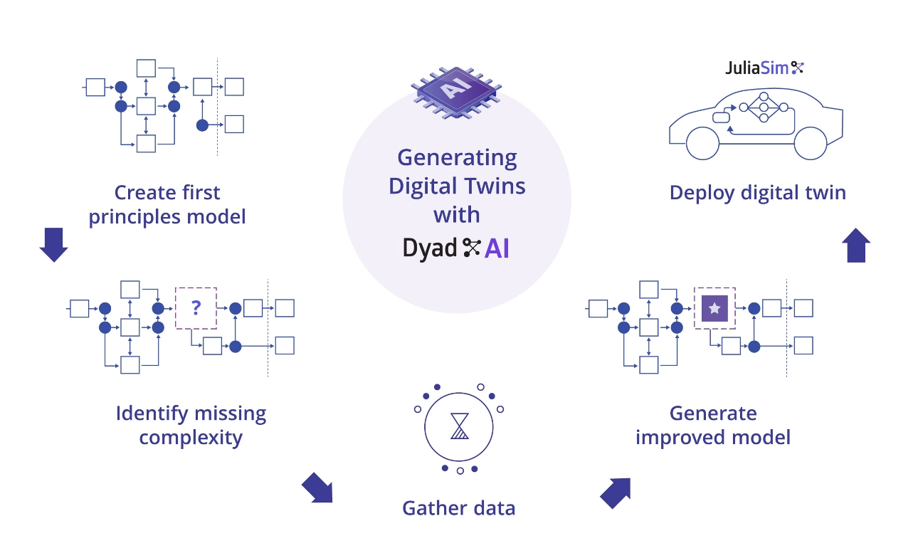
Model Discovery Analysis

Universal Differential Equations (UDEs)^[1] have emerged as a promising approach for integrating experimental data into mechanistic models via neural networks.

In this analysis, we make the neural network available as a component that can be plugged in to your existing model. You can then train that neural network using the NNTrainingAnalysis, and then estimate the possible equations that the neural network encodes using the SymbolicRegressionUDEAnalysis.

While the original UDE methodology was developed for systems of ordinary differential equations, acausal modeling presents a different challenge: we begin with differential-algebraic equations (DAEs) for each component, which are then condensed through structural simplification into a final DAE system for solution.

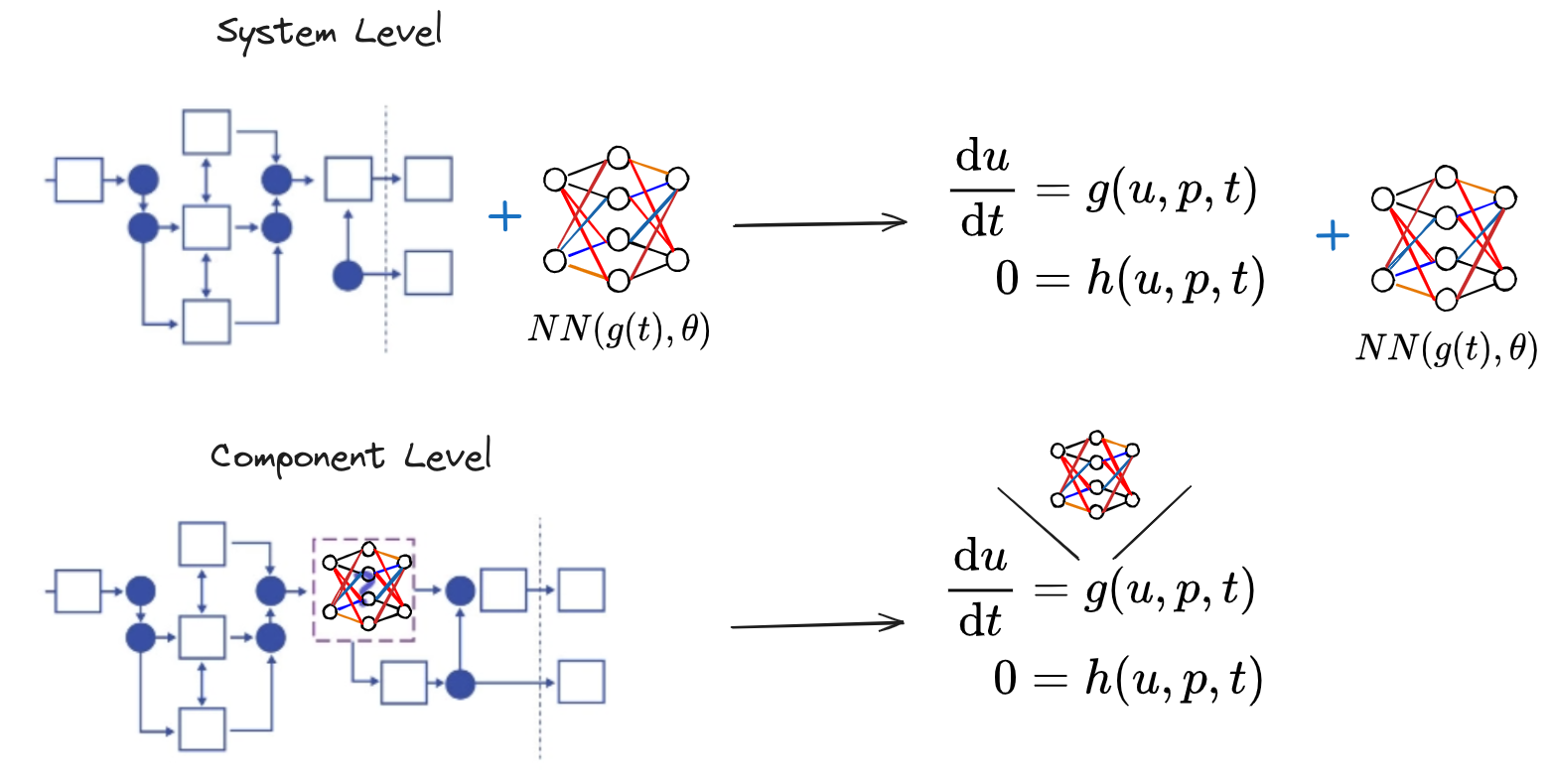
When formulating UDEs in the DAE context, we can operate at two different stages: before structural simplification (component UDE formulation) or after simplification on the resulting DAE system (system UDE formulation).

The component UDE formulation offers significant advantages. By representing the model discovery process at the block component level, we can target specific, deeply nested parts of a model while maximizing reuse of existing structural information. This approach ensures that discovered models remain expressible in the same format as the original model.

Dyad's component UDE analysis enables symbolic representation of neural networks at the block diagram level, allowing us to leverage existing system structure knowledge throughout the model discovery process.

Method Overview

We will embed a (single) neural network inside the system (represented as NeuralNetworkBlock), such that the predictions or the outputs of the neural network affect the dynamics in the desired way based on its inputs.

The Dyad compiler uses the physical description of the system, which maps to the block diagram representation, to generate a system of differential-algebraic equations via structural simplification:

$$\begin{array}{rl}{x}^{\prime }& =f(x,y,p,t)\\ 0& =g(x,y,p,t)\end{array}$$

For the component UDE model discovery analysis, we would like to perform a transformation on the system before structural simplification. In this case the system is represented by several systems of DAEs that are connected to each other. These systems can be also represented graphically via block diagrams, where each block is a potentially nested system of DAEs. When we perform the system transformation, we will embed a (single) neural network inside the system (represented as NeuralNetworkBlock), such that the predictions or the outputs of the neural network affect the dynamics in the desired way based on its inputs.

The NeuralNetworkBlock is represented as the following nonlinear system

$$outputs=NN(inputs,n{n}_p)$$

where inputs and outputs are vector variables that can be used throughout the system as desired and nn_p are the parameters of the neural network.

After we assemble the system and structurally simplify it, we will obtain a new system,

$$\begin{array}{rl}{x}^{\prime }& =f_{new}(x,y,p,t)\\ 0& =g_{new}(x,y,p,t)\end{array}$$

If we use $z(t,p)$ to denote the function of the state $[x(t,p),y(t,p)]$ for which we have data $d(t_i)$ at time points $t_i$, the goal is to find the parameters $n{n}_p$, a subset of $p$, such that $z(t_i,p\ast )\approx d(t_i)$. A nonlinear optimization is then performed to find the minimizer of $L$. In particular, gradient-based optimization using automatic differentiation and adjoint methods is used to do this fast and robustly.

Example Workflow

To run a model discovery analysis, we need a model and some data that corresponds to the behaviour that we would want from it. In this example we will consider a simple thermal system where we know part of the structure, but not enough to account for the behaviour of the system. We will add a neural network to the system, train it and then perform symbolic regression to recover possible candidate terms for the missing physics.

This example requires the following julia packages to be installed in the current environment. Use the Julia REPL to add them:

using Pkg
Pkg.add(["ThermalComponents", "BlockComponents", "DyadData", "DyadModelDiscovery"])

Let's first create the starting model in Dyad. If you already have a component library, you can add this into a new .dyad file in the dyad folder, otherwise you need to create a new component library via the Command Palette in VS Code (⇧ ⌘ P on MacOS, Ctrl-Shift-P on Windows). See the getting started instructions for more details.

Dyad code

A common issue in modeling is failing to account for all the possible ways in which a system could be storing energy, or otherwise have memory. Such behaviour is encoded by additional state variables that might be missing in a model, and thus it would not match up with the observed behavior. In this example we will study the case of a thermal capacitance for a plate, but other scenarios include elastic energy stored in parasitic flexibilities in mechanical systems, parasitic capacitance and inductance in electrical circuits, time delays in digital communication etc.

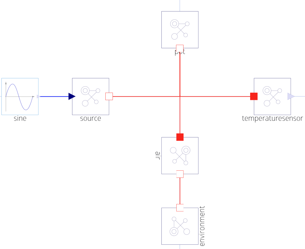
In the following we consider a pot that is being heated and some real world measurements of that system. But the dynamics of the initial model does not match the data! Let's use UDEs to discover those dynamics.

We can now add the following Dyad code describing a pot (modelled as a HeatCapacitor) that is being heated:

component SimplePot
  parameter C2::HeatCapacity = 15

  heat_input = BlockComponents.Sine(amplitude=1, frequency=1/(2*pi))
  source = ThermalComponents.PrescribedHeatFlow(T_ref=273.15)
  pot = ThermalComponents.HeatCapacitor(C=C2, T0=273.15)
  air = ThermalComponents.ThermalConductor(G=0.1)
  env = ThermalComponents.FixedTemperature(T=293.15)
  Tsensor = ThermalComponents.TemperatureSensor()

  relations
    connect(heat_input.y, source.Q)
    connect(source.node, pot.node)
    connect(pot.node, Tsensor.node)
    connect(pot.node, air.node_a)
    connect(air.node_b, env.node)
end

analysis SimplePotTransient
  extends TransientAnalysis(stop=100.0)
  model = SimplePot()
end

Let's start by running a transient analysis for the above model and check how it compares against the desired system behaviour.

using DyadInterface, DyadData, Plots

sol0 = SimplePotTransient()
model = artifacts(sol0, :SimplifiedSystem)
data = DyadDataset("juliasimtutorials", "potplate", independent_var = "timestamp", dependent_vars = ["pot.T(t)"])
df = build_dataframe(data)
plt = plot(sol0, idxs=model.pot.T)
scatter!(plt, df.timestamp, df."pot.T(t)"; label = "Real data")
plt

With the component UDE approach, we want to add a new component in the model that would be connected between the source and the pot such that we can use it to discover the missing physics. To this end, we will build a ThermalNN component that adds a new state in the system (x) that is prescribed by the output of the neural network, but it also incorporates physics knowledge about the system by formulating the component as something that outputs a heat flow rate based on some scaled input temperatures.

component ThermalNN
  structural parameter n_input::Integer = 2
  structural parameter n_output::Integer = 1
  nn = DyadModelDiscovery.NeuralNetworkBlock(n_input=n_input, n_output=n_output, chain=DyadModelDiscovery.multi_layer_feed_forward(
            n_input, n_output, depth = 1, width = 4))

  parameter T0::Temperature = 273.15
  parameter T_range::Temperature = 30
  # This is a unit conversion factor
  parameter C1::HeatCapacity = 1

  node_a = Node()
  node_b = Node()

  relations
    # This is some initial setup for the block
    # to connect its ports.
    initial node_a.T = T0
    guess node_a.Q = 0.0

    # The neural network operates in a specific range of numbers (0-1) for its inputs.
    # You should normalize your inputs to that range.  This requires that you know
    # a reasonable range of values that your inputs can take.
    nn.inputs[1] = (node_a.T - T0) / T_range
    nn.inputs[2] = (node_b.T - T0) / T_range

    # This is where we connect the neural network's output.
    # Note that it is outputting heat flow here,
    # and we are injecting it such that the derivative should be 0 at steady state, i.e., the component is conservative.
    # Here, there is a feedback loop since one of the inputs is `node_a.T`
    # and the output is related to `der(node_a.T)`.
    # The neural network is learning and encoding a new state here.
    C1 * der(node_a.T) = node_a.Q - nn.outputs[1]
    nn.outputs[1] + node_b.Q = 0

end

component NeuralPot
  parameter C2::Real = 15

  heat_input = BlockComponents.Sine(amplitude=1, frequency=1/(2*pi))
  source = ThermalComponents.PrescribedHeatFlow(T_ref=273.15)
  pot = ThermalComponents.HeatCapacitor(C=C2, T0=273.15)
  air = ThermalComponents.ThermalConductor(G=0.1)
  env = ThermalComponents.FixedTemperature(T=293.15)
  Tsensor = ThermalComponents.TemperatureSensor()
  thermal_nn = ThermalNN()

  relations
    connect(heat_input.y, source.Q)
    connect(pot.node, Tsensor.node)
    connect(pot.node, air.node_a)
    connect(air.node_b, env.node)
    connect(source.node, thermal_nn.node_a)
    connect(thermal_nn.node_b, pot.node)
end

analysis NeuralPotTransient
  extends TransientAnalysis(stop=100.0)
  model = NeuralPot()
end

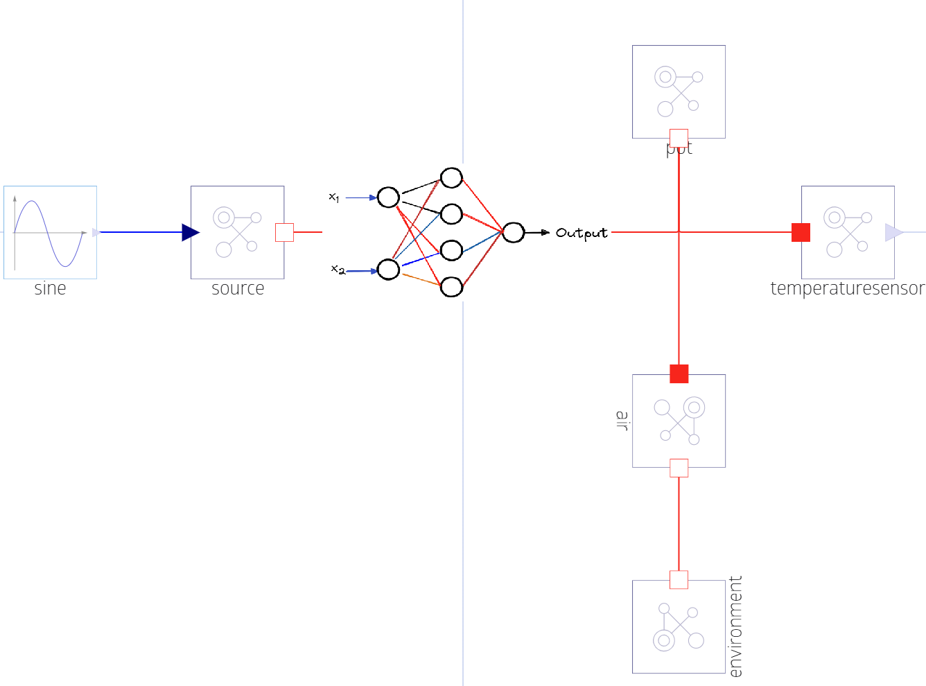
After building the ThermalNN component, we assemble the system and then define a transient analysis. Before starting the training of the neural network, we should first make sure that the augmented system is in a configuration where we can define a finite and (relatively small) loss function value.

r0 = NeuralPotTransient()
plot(r0; title = "Pre-training results")

Now that we have a reasonable starting point, we can start training the network. First we will define how to train the embedded neural network using the NNTrainingAnalysis

using DyadData: DyadDataset

analysis NeuralPotTrainingAnalysis
  extends DyadModelDiscovery.NNTrainingAnalysis(
    data=DyadData.DyadDataset("juliasimtutorials", "potplate", independent_var = "timestamp", dependent_vars = ["pot.T(t)"]),
    depvars_names=["pot.T"], alg = "Tsit5", calibration_alg="SingleShooting",
    optimizer="Adam", optimizer_maxiters=10000, network_component="thermal_nn.nn", results_path="r1.csv")
  model = NeuralPot()
end

And after that that, we switch to julia to do the training by running the analysis

r = NeuralPotTrainingAnalysis()

Calibration Analysis solution for NNTrainingAnalysis: Calibration result computed in 4 minutes and 29 seconds. Final objective value: 0.00124572.
Optimization ended with Default Return Code and returned.

┌────────────────────┬────────────────────┬────────────────────┬────────────────
│ thermal_nn₊nn₊p[1] │ thermal_nn₊nn₊p[2] │ thermal_nn₊nn₊p[3] │ thermal_nn₊nn ⋯
├────────────────────┼────────────────────┼────────────────────┼────────────────
│            1.69389 │           -3.78661 │            -2.6045 │           -2. ⋯
└────────────────────┴────────────────────┴────────────────────┴────────────────
                                                              34 columns omitted

We can now check the training results are satisfactory by inspecting artifacts such as the convergence plot

artifacts(r, :ConvergencePlot)

and looking at the simulation results with

sol = artifacts(r, :CalibratedSimulation)

retcode: Success
Interpolation: 1st order linear
t: 124-element Vector{Float64}:
   0.0
   0.12379779297215558
   0.3455862300046023
   0.6117734313827521
   0.9467695063503542
   1.340082096653101
   1.8099335887227146
   2.3837354672927185
   3.0759311456753737
   3.6786388391112745
   ⋮
  93.70314605357188
  94.61439117543479
  95.39978611258847
  96.2523916609586
  97.2396752711679
  98.03961262342023
  98.87499229893011
  99.7244805066473
 100.0
u: 124-element Vector{Vector{Float64}}:
 [273.15, 273.15]
 [273.15729322482906, 273.16652354357456]
 [273.2073763878235, 273.19614148234336]
 [273.3156154195921, 273.23245300312834]
 [273.4976091396733, 273.2803706532467]
 [273.73109479087367, 273.34053582778137]
 [273.97188082240575, 273.4174500428582]
 [274.12317221132923, 273.5152909092424]
 [274.03140920322187, 273.62984978347544]
 [273.7519914673216, 273.71748806885796]
 ⋮
 [281.30910499021894, 282.03942859054376]
 [281.7457106610697, 282.072514215342]
 [282.3254773727679, 282.1268604345655]
 [282.79497288671126, 282.213114475086]
 [282.7932608304108, 282.3227474256941]
 [282.39841738409746, 282.3937518666136]
 [281.91787374198447, 282.4381632339513]
 [281.71002951805775, 282.4608057146627]
 [281.7426783924642, 282.4669055754612]

After we are satisfied with the results, we can export them, such that we can use the neural network as a dataset for performing symbolic regression.

artifacts(r, :ResultsExport)

"r1.csv"

We then describe the analysis in Dyad

analysis NeuralPotUDEAnalysis
  extends DyadModelDiscovery.SymbolicRegressionUDEAnalysis(
    data=DyadData.DyadDataset("juliasimtutorials", "potplate", independent_var = "timestamp", dependent_vars = ["pot.T(t)"]),
    depvars_names=["pot.T"], alg="Tsit5", network_component="thermal_nn.nn", training_result="r1.csv",
    maxdepth = 5, maxsize=7)
  model = NeuralPot()
end

And then we go back to julia to run the analysis with

result = NeuralPotUDEAnalysis()

System level UDE results for SymbolicRegressionUDEAnalysis: 4 candidate models
┌─────────────────────────────────────────────────────────────┬─────────────┐
│ candidate terms for (NeuralPot₊thermal_nn₊nn₊outputs(t))[1] │  cost value │
│                                               Symbolics.Num │         Any │
├─────────────────────────────────────────────────────────────┼─────────────┤
│                        p₁*((inputs(t))[1] - (inputs(t))[2]) │ 0.000148277 │
│                 p₂*((inputs(t))[1] - ((inputs(t))[2] - p₁)) │ 0.000315652 │
│                                                          p₁ │    0.434279 │
│                             (inputs(t))[1] - (inputs(t))[2] │     1.10406 │
└─────────────────────────────────────────────────────────────┴─────────────┘
┌───────────────────────┬───────────────────────┐
│            parameters │              defaults │
│ Vector{Symbolics.Num} │                Vector │
├───────────────────────┼───────────────────────┤
│               Num[p₁] │             [29.9862] │
│           Num[p₁, p₂] │ [1.86196e-5, 29.9921] │
│               Num[p₁] │          [-0.0848182] │
│                 Num[] │                 Any[] │
└───────────────────────┴───────────────────────┘

Looking at the results, we can see a table of candidate models, where we can compare them based on how well they fit our data. Looking at the top candidate, we can observe that the candidate terms that would replace the neural network would be directly proportional with the difference of the neural network inputs. Going back to the definition of the ThermalNN component, we see that the inputs are the temperatures on each side of the component. Since the component outputs a heat flow rate, this also makes physical sense.

Further Reading

---

1. C. Rackauckas et al., “Universal Differential Equations for Scientific Machine Learning,” arXiv:2001.04385 [cs, math, q-bio, stat], Jan. 2020, Accessed: Feb. 09, 2020. [Online]. Available: http://arxiv.org/abs/2001.04385 ↩︎