
Sampled-Data Systems
A sampled-data system contains both continuous-time and discrete-time parts — most often a continuous-time plant model together with a discrete-time control system running at a fixed rate. This page covers what is needed on top of ordinary discrete-time modeling: the two operators that move signals between the domains, and how to think about them.
Sample and hold
The two domains describe signals on different time sets, and that is the whole source of the difficulty:
A continuous-time signal has a value at every instant of the simulated interval.
A discrete-time signal has a value only at the ticks of its associated clock. Between ticks it is not "the previous value" — it is simply not defined. Asking what a clocked signal equals halfway between two ticks is not a meaningful question.
Two operators bridge the gap, and they are not symmetric.
Sampler restricts a continuous-time signal to the tick times of a clock. It throws information away: whatever the signal did between ticks is not represented in the result. You can think of sampling as taking a measurement of the sampled signal when the clock ticks.
ZeroOrderHold goes the other way. A discrete-time signal has no values between ticks, so producing a continuous-time signal from it requires interpolation: the sequence of samples is extended onto the continuous-time axis. Zero-order hold is the simplest such rule — keep the last sample constant until the next tick — which is what a digital-to-analog converter driven by a register physically does, and why it is the default. Other interpolations (linear, higher-order) are other choices of the same kind of rule.
Two consequences follow from the hold being an interpolation rather than a recovery:
The continuous-time signal downstream of a hold is a model of what the hardware does between updates. If the real converter behaves differently, the model is wrong there in a way no choice of sample rate fixes.
The hold, not the sampler, is where the loop's phase lag comes from. Holding a value for one period delays it by half a period on average, which is why discretizing a controller costs phase margin.
Connecting across the boundary
A time-varying continuous signal may not be connected directly to a clocked input — it has to pass through a Sampler first. This is why the example below routes its Step source through a sampler before the signal enters the discrete-time partition. A time-invariant signal such as a Constant is fine to connect directly, because it has the same value at every tick.
In the other direction, a clocked signal reaching a continuous-time component must pass through a ZeroOrderHold.
Troubleshooting
| Symptom | Cause and fix |
|---|---|
Attempted to combine clocked value with continuous-time value | A continuous-time signal reached a clocked equation, or a clocked signal reached a continuous-time one. Insert a Sampler or a ZeroOrderHold in the appropriate direction. |
For clock errors that do not involve the continuous-time domain, see Troubleshooting clock errors.
Reading results across the boundary
The idioms for plotting and indexing clocked variables are the same as for a purely discrete-time model — see Reading results.
A ZeroOrderHold output is stored on the clock partition of the signal that feeds it, so it is read like any other clocked variable: in a model with connect(controller.y, zoh.u), sol[model.zoh.y] and sol(t; idxs = model.zoh.y) return the held trace and agree with model.controller.y. The same holds for any variable defined by a hold.
Linearization of sampled-data systems
Linearization of discrete-time and sampled-data systems can be performed using frequency-response analysis (FRA) in DyadControlSystems. FRA amounts to simulating a system with wide-spectrum inputs and computing the linear small-signal transfer function using techniques from the field of system identification.
FRA is used here because forward-mode automatic differentiation cannot currently propagate through a clocked update, so the analytic linearization available for purely continuous models does not apply to a partition that contains discrete-time logic. FRA sidesteps this by working from simulation data only.
A complete example
Below, we model a simple continuous first-order system called plant that is controlled using a discrete-time controller. The reference signal is filtered using a discrete-time exponential filter before being fed to the controller. We use a Sampler driven by a PeriodicClock to sample the plant output, and ZeroOrderHold to convert the discrete controller output back to continuous time. Download as a Dyad projectclocks.zipOpen in Dyad Studio
"""
A simple sampled-data control system with a continuous-time first-order plant
and a discrete-time proportional controller with reference filtering.
"""
example component SampledDataDemo
  "Continuous-time plant: dx/dt = -x + u"
  plant = BlockComponents.Continuous.FirstOrder(k = 1, T = 1) {^plant}
  "Reference step at t=5"
  ref = BlockComponents.Sources.Step(height = 1, start_time = 5) {^ref}
  "Sample the reference before it enters the discrete-time partition"
  ref_sampler = DiscreteComponents.Sampler() {^ref_sampler}
  "Sample the plant output at 2 Hz"
  sampler = DiscreteComponents.Sampler() {^sampler}
  clock = DiscreteComponents.PeriodicClock(dt = 0.5) {^clock}
  "Discrete-time exponential reference filter"
  filt = DiscreteComponents.ExponentialFilter(a = 0.393) {^filt}
  "Proportional controller (discrete-time)"
  err = BlockComponents.Math.Add(k2 = -1) {^err}
  gain = BlockComponents.Math.Gain(k = 1) {^gain}
  "Hold controller output for the plant"
  zoh = DiscreteComponents.ZeroOrderHold() {^zoh}
relations
  initial plant.x = 1
  # Reference filtering. The continuous-time reference is sampled before it enters
  # the discrete-time partition that `filt` belongs to.
  connect(ref.y, ref_sampler.u) {^id8}
  connect(ref_sampler.y, filt.u) {^id15}
  # Error = filtered_ref - sampled_plant
  connect(filt.y, err.u1) {^id9}
  connect(sampler.y, err.u2, clock.y) {^id10}
  # Controller
  connect(err.y, gain.u) {^id11}
  # D/A conversion and plant
  connect(gain.y, zoh.u) {^id12}
  connect(zoh.y, plant.u) {^id13}
  # Feedback sampling
  connect(plant.y, sampler.u) {^id14}
metadata {
  "_links": {
    "plant": {
      "Dyad": {
        "placement": {
          "diagram": {"iconName": "default", "x1": 40, "y1": 140, "x2": 240, "y2": 340, "rot": 0}
        },
        "tags": []
      }
    },
    "ref": {
      "Dyad": {
        "placement": {
          "diagram": {"iconName": "default", "x1": -230, "y1": -220, "x2": -30, "y2": -20, "rot": 0}
        },
        "tags": []
      }
    },
    "ref_sampler": {
      "Dyad": {
        "placement": {
          "diagram": {"iconName": "default", "x1": 40, "y1": -220, "x2": 240, "y2": -20, "rot": 0}
        },
        "tags": []
      }
    },
    "sampler": {
      "Dyad": {
        "placement": {
          "diagram": {"iconName": "default", "x1": 300, "y1": 140, "x2": 500, "y2": 340, "rot": 0}
        },
        "tags": []
      }
    },
    "clock": {
      "Dyad": {
        "placement": {
          "diagram": {"iconName": "default", "x1": 300, "y1": 380, "x2": 500, "y2": 580, "rot": 0}
        },
        "tags": []
      }
    },
    "filt": {
      "Dyad": {
        "placement": {
          "diagram": {"iconName": "default", "x1": 300, "y1": -220, "x2": 500, "y2": -20, "rot": 0}
        },
        "tags": []
      }
    },
    "err": {
      "Dyad": {
        "placement": {
          "diagram": {"iconName": "default", "x1": 570, "y1": 80, "x2": 770, "y2": 280, "rot": 0}
        },
        "tags": []
      }
    },
    "gain": {
      "Dyad": {
        "placement": {
          "diagram": {"iconName": "default", "x1": 830, "y1": 80, "x2": 1030, "y2": 280, "rot": 0}
        },
        "tags": []
      }
    },
    "zoh": {
      "Dyad": {
        "placement": {
          "diagram": {"iconName": "default", "x1": 1078, "y1": 80, "x2": 1278, "y2": 280, "rot": 0}
        },
        "tags": []
      }
    },
    "id8": {"Dyad": {"edges": [{"S": 1, "M": [], "E": 2}], "renderStyle": "standard"}},
    "id9": {
      "Dyad": {
        "edges": [{"S": 1, "M": [{"x": 540, "y": -120}, {"x": 540, "y": 120}], "E": 2}],
        "renderStyle": "standard"
      }
    },
    "id10": {"Dyad": {"edges": [{"S": 1, "M": [], "E": 2}], "renderStyle": "standard"}},
    "id11": {"Dyad": {"edges": [{"S": 1, "M": [], "E": 2}], "renderStyle": "standard"}},
    "id12": {"Dyad": {"edges": [{"S": 1, "M": [], "E": 2}], "renderStyle": "standard"}},
    "id13": {
      "Dyad": {
        "edges": [
          {
            "S": 1,
            "M": [
              {"x": 1300, "y": 180},
              {"x": 1300, "y": 650},
              {"x": 0, "y": 650},
              {"x": 0, "y": 240}
            ],
            "E": 2
          }
        ],
        "renderStyle": "standard"
      }
    },
    "id14": {"Dyad": {"edges": [{"S": 1, "M": [], "E": 2}], "renderStyle": "standard"}},
    "id15": {"Dyad": {"edges": [{"S": 1, "M": [], "E": 2}], "renderStyle": "standard"}}
  }
}
end

analysis SampledDataDemoAnalysis
  extends TransientAnalysis(stop = 15.0)
  model = SampledDataDemo()
end
We can now simulate the system:
using Plots
plot(SampledDataDemoAnalysis())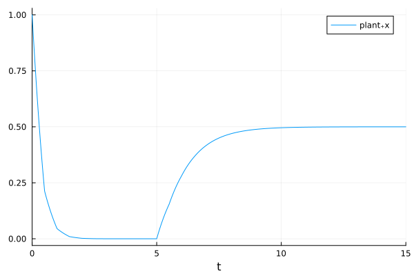
Known limitations
Beyond the discrete-time limitations, these apply to sampled-data models specifically.
No automatic differentiation through a clocked partition. Forward-mode AD does not propagate through the discrete-time update, so the analytic linearization available for purely continuous-time models does not apply; use FRA instead.
FMU export rejects models containing events, which includes clocked models.
A model containing a continuous-time partition cannot be compiled to a standalone program. See Code Generation and Deployment.
See also
Discrete-Time Modeling — clocks, the synchronous programming model, difference equations and multi-rate systems
Measurement Noise and Corruption — sensor imperfections, quantization and AD effects
DC Motor with PI Controller — a continuous-time model converted to sampled-data control, then to cascade control
On-Off Controller — a relay controller with hysteresis
Sliding-Mode Control — a discrete-time super-twisting controller
Discretizing Continuous-Time Linear Systems —
c2dand the choice of discretization methodFrequency-response analysis — linearizing a sampled-data system
ControlSystems.jl: Analysis of sampled-data systems — how the hold interacts with continuous-time frequency-domain analysis
DyadControlSystems — controller design, MPC and state estimation