TUTORIAL

Sliding-Mode Control

This example demonstrates how to model a system with a discrete-time sliding-mode controller (SMC) in Dyad. The system consists of a second-order plant with a disturbance and a SuperTwistingSMC controller. The controller is implemented as a discrete-time system, and the plant is modeled as a continuous-time system.

Background

When designing an SMC controller, we must choose a switching function that produces the sliding variable  . The sliding surface   must be chosen such that the sliding variable exhibits desirable properties, i.e., converges to the desired state with stable dynamics. The control law is chosen to drive the system from any state    to the sliding surface  . The sliding surface is commonly chosen as an asymptotically stable system with order equal to  , where is the dimension of the state in the system to be controlled, and is the number of inputs.

Since the dynamics in this example is of relative degree  , we will choose a switching surface corresponding to a stable first-order system (  ). We will choose the system

which yields the switching variable   , where    is the tracking error.

Implementation

The sliding variable is computed from the sampled signals using block diagram components. The plant position is sampled (with AD effects for realism), filtered through an ExponentialFilter, and differentiated using a DiscreteDerivative to estimate velocity. The position and velocity errors relative to the reference signals are summed to form the sliding variable     , which is fed to the SuperTwistingSMC controller. Download as a Dyad projectSMC.zipOpen in Dyad Studio›

"""
Test component that validates the SuperTwistingSMC sliding mode controller.

A second-order plant tracks a sinusoidal reference `qr = sin(2t)` under disturbance
`d = 2 + 2sin(3t) + sin(5t)`. The plant position is sampled and differentiated to estimate
velocity. The sliding variable `s = (xd - qdr) + (x - qr)` is computed from the sampled
signals and fed to the super-twisting controller. The controller output is held by a ZOH
and summed with the disturbance before driving the plant.
"""
test component TestSlidingModeControl
  "Plant"
  secondorder = BlockComponents.Continuous.SecondOrder() {^secondorder}
  "Velocity estimation via discrete derivative of sampled position"
  dd_xd = DiscreteComponents.DiscreteDerivative(initialization = DiscreteComponents.InitialCondition.InitialOutput(y0 = 0.01)) {^dd_xd}
  "Reference: qr = sin(2t), qdr = 2*cos(2t)"
  sine_ref = BlockComponents.Sources.Sine(amplitude = 1, frequency = 0.31831) {^sine_ref}
  cosine_refd = BlockComponents.Sources.Cosine(amplitude = 2, frequency = 0.31831) {^cosine_refd}
  ps_qr = DiscreteComponents.Sampler() {^ps_qr}
  ps_qdr = DiscreteComponents.Sampler() {^ps_qdr}
  zoh = DiscreteComponents.ZeroOrderHold() {^zoh}
  "Disturbance: 2 + 2*sin(3t) + sin(5t)"
  constant_dist = BlockComponents.Sources.Constant(k = 2) {^constant_dist}
  sine_dist1 = BlockComponents.Sources.Sine(amplitude = 2, frequency = 0.477465) {^sine_dist1}
  sine_dist2 = BlockComponents.Sources.Sine(amplitude = 1, frequency = 0.795775) {^sine_dist2}
  "Sliding variable computation: s = (x - qr) + (xd_est - qdr)"
  err_pos = BlockComponents.Math.Add(k2 = -1) {^err_pos}
  err_vel = BlockComponents.Math.Add(k2 = -1) {^err_vel}
  """
  sliding surface
  
  Combines two input signals by multiplying each by its respective gain parameter and adding the results. The output
  is calculated as
  
  ```math
  y = k1 \cdot u1 + k2 \cdot u2

where k1 and k2 are configurable gain factors that determine the weight of each input in the sum. """ sliding_surface = BlockComponents.Math.Add() {^sliding_surface} "Control + disturbance → plant" add_ctrl = BlockComponents.Math.Add() {^add_ctrl} add3 = BlockComponents.Math.Add3() {^add3} smc = DiscreteComponents.SuperTwistingSMC(k = 50) {^smc} periodicclock = DiscreteComponents.PeriodicClock(dt = 0.01) {^periodicclock} samplewithadeffects = DiscreteComponents.SampleWithADEffects(y_min = -3, y_max = 3, bits = 12, sigma = 0.01) {^samplewithadeffects} exponentialfilter = DiscreteComponents.ExponentialFilter(a = 0.2, initialization = DiscreteComponents.InitialCondition.InitialOutput(y0 = -1)) {^exponentialfilter} variable disturbance::Real relations initial secondorder.x = -1 initial secondorder.xd = 0

Sample references

connect(sine_ref.y, ps_qr.u) {^id20} connect(cosine_refd.y, ps_qdr.u) {^id21} connect(zoh.y, add_ctrl.u1) {^id22} connect(add_ctrl.y, secondorder.u) {^id23} connect(dd_xd.y, err_vel.u1) {^id24} connect(ps_qdr.y, err_vel.u2) {^id25} connect(err_pos.y, sliding_surface.u1) {^id26} connect(ps_qr.y, err_pos.u2) {^id27} connect(sine_dist1.y, add3.u2) {^id28} connect(add3.y, add_ctrl.u2) {^id29} connect(err_vel.y, sliding_surface.u2) {^id30} connect(smc.s, sliding_surface.y) {^id31} connect(smc.y, zoh.u) {^id32} connect(constant_dist.y, add3.u1) {^id33} connect(sine_dist2.y, add3.u3) {^id34} connect(samplewithadeffects.u, secondorder.y) {^id35} connect(samplewithadeffects.y, periodicclock.y, exponentialfilter.u) {^id36} connect(exponentialfilter.y, dd_xd.u, err_pos.u1) {^id37} metadata { "Dyad": { "tests": { "case1": {"stop": 6, "expect": {"signals": ["secondorder.y", "smc.y"]}} }, "doc": {"behavior": false} }, "_links": { "secondorder": { "Dyad": { "placement": { "diagram": {"iconName": "default", "x1": 1020, "y1": 660, "x2": 1120, "y2": 760, "rot": 0} }, "tags": [] } }, "dd_xd": { "Dyad": { "placement": { "diagram": {"iconName": "default", "x1": 140, "y1": 850, "x2": 40, "y2": 950, "rot": 90} }, "tags": [] } }, "sine_ref": { "Dyad": { "placement": { "diagram": {"iconName": "default", "x1": -200, "y1": 480, "x2": -100, "y2": 580, "rot": 0} }, "tags": [] } }, "cosine_refd": { "Dyad": { "placement": { "diagram": {"iconName": "default", "x1": -200, "y1": 690, "x2": -100, "y2": 790, "rot": 0} }, "tags": [] } }, "ps_qr": { "Dyad": { "placement": { "diagram": {"iconName": "default", "x1": -70, "y1": 480, "x2": 30, "y2": 580, "rot": 0} }, "tags": [] } }, "ps_qdr": { "Dyad": { "placement": { "diagram": {"iconName": "default", "x1": -70, "y1": 690, "x2": 30, "y2": 790, "rot": 0} }, "tags": [] } }, "zoh": { "Dyad": { "placement": { "diagram": {"iconName": "default", "x1": 690, "y1": 690, "x2": 790, "y2": 790, "rot": 0} }, "tags": [] } }, "constant_dist": { "Dyad": { "placement": { "diagram": {"iconName": "default", "x1": 520, "y1": 280, "x2": 620, "y2": 380, "rot": 0} }, "tags": [] } }, "sine_dist1": { "Dyad": { "placement": { "diagram": {"iconName": "default", "x1": 520, "y1": 410, "x2": 620, "y2": 510, "rot": 0} }, "tags": [] } }, "sine_dist2": { "Dyad": { "placement": { "diagram": {"iconName": "default", "x1": 520, "y1": 540, "x2": 620, "y2": 640, "rot": 0} }, "tags": [] } }, "err_pos": { "Dyad": { "placement": { "diagram": {"iconName": "default", "x1": 150, "y1": 660, "x2": 250, "y2": 560, "rot": 0} }, "tags": [] } }, "err_vel": { "Dyad": { "placement": { "diagram": {"iconName": "default", "x1": 150, "y1": 820, "x2": 250, "y2": 720, "rot": 0} }, "tags": [] } }, "sliding_surface": { "Dyad": { "placement": { "diagram": {"iconName": "default", "x1": 360, "y1": 690, "x2": 460, "y2": 790, "rot": 0} }, "tags": [] } }, "add_ctrl": { "Dyad": { "placement": { "diagram": {"iconName": "default", "x1": 880, "y1": 760, "x2": 980, "y2": 660, "rot": 0} }, "tags": [] } }, "add3": { "Dyad": { "placement": { "diagram": {"iconName": "default", "x1": 690, "y1": 410, "x2": 790, "y2": 510, "rot": 0} }, "tags": [] } }, "smc": { "Dyad": { "placement": { "diagram": {"iconName": "default", "x1": 520, "y1": 690, "x2": 620, "y2": 790, "rot": 0} }, "tags": [] } }, "periodicclock": { "Dyad": { "placement": { "diagram": {"iconName": "default", "x1": 880, "y1": 800, "x2": 980, "y2": 900, "rot": 0} }, "tags": [] } }, "samplewithadeffects": { "Dyad": { "placement": { "diagram": {"iconName": "default", "x1": 980, "y1": 940, "x2": 880, "y2": 1040, "rot": 0} }, "tags": [] } }, "exponentialfilter": { "Dyad": { "placement": { "diagram": {"iconName": "default", "x1": 530, "y1": 940, "x2": 430, "y2": 1040, "rot": 0} }, "tags": [] } }, "id20": {"Dyad": {"edges": [{"S": 1, "M": [], "E": 2}], "renderStyle": "standard"}}, "id21": {"Dyad": {"edges": [{"S": 1, "M": [], "E": 2}], "renderStyle": "standard"}}, "id22": {"Dyad": {"edges": [{"S": 1, "M": [], "E": 2}], "renderStyle": "standard"}}, "id23": {"Dyad": {"edges": [{"S": 1, "M": [], "E": 2}], "renderStyle": "standard"}}, "id24": { "Dyad": { "edges": [{"S": 1, "M": [{"x": 90, "y": 800}], "E": 2}], "renderStyle": "standard" } }, "id25": {"Dyad": {"edges": [{"S": 1, "M": [], "E": 2}], "renderStyle": "standard"}}, "id26": { "Dyad": { "edges": [{"S": 1, "M": [{"x": 280, "y": 610}, {"x": 280, "y": 710}], "E": 2}], "renderStyle": "standard" } }, "id27": { "Dyad": { "edges": [{"S": 1, "M": [{"x": 68, "y": 530}, {"x": 68, "y": 580}], "E": 2}], "renderStyle": "standard" } }, "id28": {"Dyad": {"edges": [{"S": 1, "M": [], "E": 2}], "renderStyle": "standard"}}, "id29": { "Dyad": { "edges": [{"S": 1, "M": [{"x": 830, "y": 460}, {"x": 830, "y": 680}], "E": 2}], "renderStyle": "standard" } }, "id30": {"Dyad": {"renderStyle": "standard", "edges": [{"S": 1, "E": 2, "M": []}]}}, "id31": {"Dyad": {"edges": [{"S": 1, "M": [], "E": 2}], "renderStyle": "standard"}}, "id32": {"Dyad": {"edges": [{"S": 1, "M": [], "E": 2}], "renderStyle": "standard"}}, "id33": { "Dyad": { "renderStyle": "standard", "edges": [{"S": 1, "M": [{"x": 657.5, "y": 330}, {"x": 657.5, "y": 430}], "E": 2}] } }, "id34": { "Dyad": { "renderStyle": "standard", "edges": [{"S": 1, "M": [{"x": 657.5, "y": 590}, {"x": 657.5, "y": 490}], "E": 2}] } }, "id35": { "Dyad": { "edges": [{"S": 1, "M": [{"x": 1160, "y": 990}, {"x": 1160, "y": 710}], "E": 2}], "renderStyle": "standard" } }, "id36": { "Dyad": { "edges": [ {"S": 1, "M": [], "E": -1}, {"S": -1, "M": [{"x": 800, "y": 990}, {"x": 800, "y": 850}], "E": 2}, {"S": 3, "M": [], "E": -1} ], "junctions": [{"x": 800, "y": 990}], "renderStyle": "standard" } }, "id37": { "Dyad": { "edges": [ {"S": 1, "M": [], "E": -1}, {"S": -1, "M": [{"x": 90, "y": 990}], "E": 2}, {"S": 3, "M": [{"x": -250, "y": 640}, {"x": -250, "y": 990}], "E": -1} ], "junctions": [{"x": 90, "y": 990}], "renderStyle": "standard" } } } } end

analysis SlidingModeControlDemoAnalysis extends TransientAnalysis(stop = 10.0) model = TestSlidingModeControl() end

```julia
using Plots
result = SlidingModeControlDemoAnalysis()
using DyadInterface
model = artifacts(result, :SimplifiedSystem)
figy = plot(result; idxs = model.secondorder.y, label = "Plant position")
plot!(result; idxs = model.sine_ref.y, label = "Reference")
figu = plot(result; idxs = model.smc.y, label = "Control signal")
plot!(result; idxs = model.add3.y, label = "Disturbance")
plot(figy, figu, layout = (2, 1))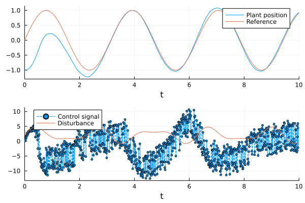

The simulation indicates that the controller is able to track the reference signal despite the presence of the disturbance. The control signal exhibits a small degree of high-frequency chattering, a common characteristic of sliding-mode controllers. The use of SampleWithADEffects and ExponentialFilter adds realistic measurement imperfections: 12-bit quantization, small Gaussian noise, and low-pass filtering of the position signal.