LIBRARY

Trajectory planning

Two methods of planning trajectories are available

• point_to_point: Generate a minimum-time point-to-point trajectory with specified start and endpoints, not exceeding specified speed and acceleration limits.

• traj5: Generate a 5th order polynomial trajectory with specified start and end points. Additionally allows specification of start and end values for velocity and acceleration.

• TrajectoryLimiters.JerkLimiter from TrajectoryLimiters.jl: Generate time-optimal trajectories with bounded jerk, acceleration and velocity using the Ruckig algorithm.

Components that make use of these trajectory generators is provided:

• KinematicPTP

• KinematicPTPBoundedJerk

• Kinematic5

These all have output connectors of type RealOutput called q, qd, qdd for positions, velocities and accelerations.

With several axes, KinematicPTP plans all axes jointly: they accelerate, cruise and decelerate in unison and reach their end position at the same time, tracing a straight line in output space. The axis that needs the most time saturates its limit, all other axes stay below theirs. KinematicPTPBoundedJerk instead time-synchronizes the axes by default, which makes them arrive together but in general along a curved path; pass phase_synchronization = true for a straight line. Kinematic5 plans each axis independently, they merely share the final time tf.

Example

Point-to-point trajectory with bounded acceleration

using MultibodyComponents, Plots
Ts = 0.001
t  = -0.5:Ts:3

q1      = [1, 1.2]      # Final point (2 DOF)
qd_max  = [0.7, 1.2]    # Max velocity (2 DOF)
qdd_max = [0.9, 1.1]    # Max acceleration (2 DOF)
q, qd, qdd = MultibodyComponents.point_to_point(t; q1, qd_max, qdd_max)

plot(t, [q qd qdd], ylabel=["\$q\$" "\$\\dot{q}\$" "\$\\ddot{q}\$"], layout=(3,1), l=2, sp=[1 1 2 2 3 3], legend=false)
hline!([qd_max' qdd_max'], l=(2, :dash), sp=[2 2 3 3], c=[1 2 1 2], legend=false)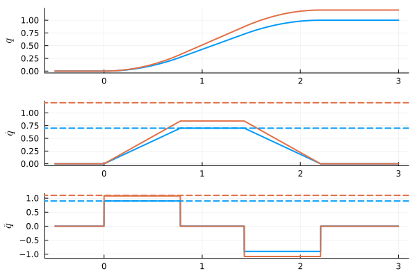

Point-to-point trajectory with bounded jerk

This kind of trajectory generator is implemented in TrajectoryLimiters.jl, it may be used as a component in a multibody model through KinematicPTPBoundedJerk.

using MultibodyComponents, Plots
Ts = 0.001
t  = -0.5:Ts:3

q1       = [1, 1.2]      # Final point (2 DOF)
qd_max   = [0.7, 1.2]    # Max velocity (2 DOF)
qdd_max  = [0.9, 1.1]    # Max acceleration (2 DOF)
qddd_max = [4.0, 4.0]    # Max jerk (2 DOF)

lims = [MultibodyComponents.JerkLimiter(; vmax=qd_max[i], amax=qdd_max[i], jmax=qddd_max[i]) for i in 1:length(q1)] # One limiter per DOF

profiles = MultibodyComponents.calculate_trajectory(lims; pf=q1)
q, qd, qdd, qddd = profiles(t)

plot(t, [q qd qdd], ylabel=["\$q\$" "\$\\dot{q}\$" "\$\\ddot{q}\$"], layout=(3,1), l=2, sp=[1 1 2 2 3 3], legend=false)
hline!([qd_max' qdd_max'], l=(2, :dash), sp=[2 2 3 3], c=[1 2 1 2], legend=false)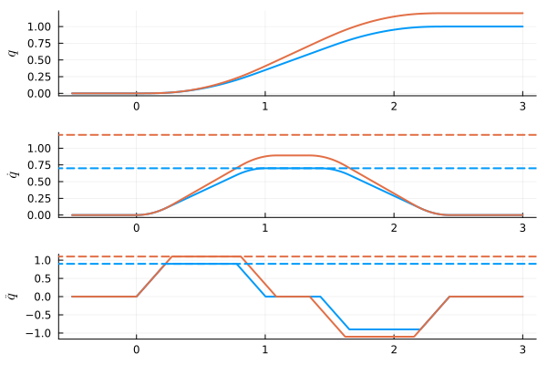

Bounded-jerk trajectory through multiple waypoints

KinematicPTPBoundedJerk can traverse a mission of several waypoints by passing a waypoints matrix, one column per waypoint. The motion comes to a full stop at every intermediate waypoint, and each segment between consecutive waypoints is an independent time-optimal jerk-limited motion. The trajectory below is that same concatenation of segments, plotted directly from the underlying profiles (dashed lines mark the interior waypoint times).

using MultibodyComponents, Plots

waypoints = [0.0 1.0 0.3 0.8]   # one axis, four waypoints (each column is a waypoint)
lim = MultibodyComponents.JerkLimiter(; vmax=1.0, amax=1.0, jmax=10.0)

# One time-optimal jerk-limited segment between each pair of consecutive waypoints,
# accumulating each segment's start time (this is what KinematicPTPBoundedJerk builds)
offsets = Float64[0.0]
profiles = map(1:size(waypoints, 2)-1) do j
    p = MultibodyComponents.calculate_trajectory([lim]; p0=waypoints[:, j], pf=waypoints[:, j+1])[1]
    push!(offsets, offsets[end] + MultibodyComponents.duration(p))
    p
end

Ts = 0.001
t  = 0:Ts:(offsets[end] + 0.2)
sample(ti) = MultibodyComponents.evaluate_at(profiles[clamp(searchsortedlast(offsets, ti), 1, length(profiles))],
                                             ti - offsets[clamp(searchsortedlast(offsets, ti), 1, length(profiles))])
traj = reduce(vcat, collect(sample(ti))' for ti in t)   # columns: q, qd, qdd, qddd

plot(t, traj[:, 1:3], ylabel=["\$q\$" "\$\\dot{q}\$" "\$\\ddot{q}\$"], layout=(3,1), l=2, sp=[1 2 3], legend=false)
vline!(offsets[2:end-1]', l=(1, :dash), c=:gray, sp=[1 2 3], legend=false)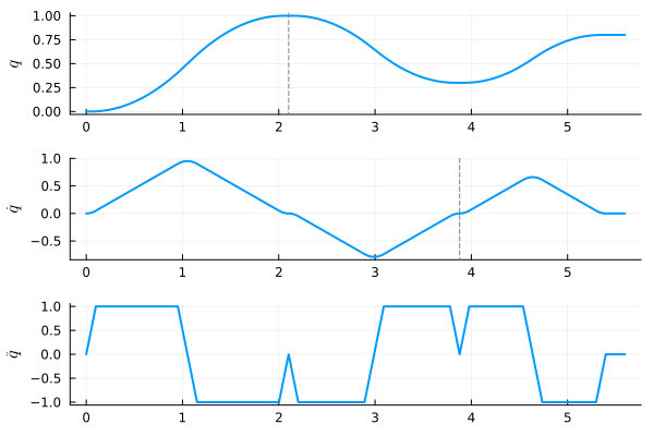

5th order polynomial trajectory

t  = 0:Ts:3
q1 = 1
q, qd, qdd = MultibodyComponents.traj5(t; q1)

plot(t, [q qd qdd], ylabel=["\$q\$" "\$\\dot{q}\$" "\$\\ddot{q}\$"], layout=(3,1), l=2, legend=false)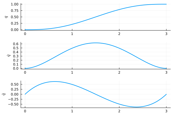

Docstrings

• MultibodyComponents.KinematicPTPBoundedJerk
• MultibodyComponents.point_to_point
• MultibodyComponents.prepare_trajectory_planner
• MultibodyComponents.ptp_trajectory
• MultibodyComponents.traj5
• MultibodyComponents.traj5
• MultibodyComponents.traj5_trajectory

MultibodyComponents.KinematicPTPBoundedJerk Method

KinematicPTPBoundedJerk(; name, q0=0, q1=1, qd_max=1, qdd_max=1, qddd_max=10, phase_synchronization=false, waypoints=nothing)

A component emitting a time-optimal point-to-point trajectory with bounded velocity, acceleration, and jerk, generated using JerkLimiter from TrajectoryLimiters.jl.

By default the motion goes from q0 to q1. To traverse a mission of several waypoints, pass a waypoints matrix of size nout × nwp whose columns are the successive waypoints (the first column is the start, the last the target); this overrides q0/q1. The motion comes to a full stop (zero velocity and acceleration) at every intermediate waypoint, and each segment between consecutive waypoints is an independent time-optimal jerk-limited motion. The segments are concatenated on the time axis, so the output follows segment 1 for its duration, then segment 2, and so on, holding the final waypoint after the mission completes.

When multiple axes are specified, the per-segment trajectories are by default time-synchronized so all axes reach the next waypoint at the same time. Time synchronization does not keep the axis velocities proportional to each other, so the path traced in output space is in general not a straight line. With phase_synchronization = true, the axes are phase-synchronized (synchronization = :phase in TrajectoryLimiters): the velocity direction is constant within each segment and the path is an exact straight line between consecutive waypoints, at the same time-optimal duration as time synchronization.

Phase synchronization requires the per-axis limits to admit the straight-line profile. This always holds when all axes share the same limits. With differing per-axis limits where different axes bind different limit types (e.g. one axis velocity-bound and another jerk-bound), no straight-line profile exists at the synchronized duration and an error is thrown; making the limits equal across axes, or proportional to each axis's travel distance, restores feasibility.

Arguments

• name: Name of the component

• q0: Initial position (scalar or vector), used when waypoints is not given

• q1: Final position (scalar or vector), used when waypoints is not given

• qd_max: Maximum velocity (scalar or vector)

• qdd_max: Maximum acceleration (scalar or vector)

• qddd_max: Maximum jerk (scalar or vector)

• phase_synchronization: Phase-synchronize the axes (straight line in output space)

• waypoints: Optional nout × nwp matrix whose columns are the waypoints to traverse; overrides q0/q1 when given. Requires at least two columns.

Outputs

• q: Position

• qd: Velocity

• qdd: Acceleration

• qddd: Jerk

MultibodyComponents.point_to_point Method

q, qd, qdd, t_end = point_to_point(time; q0=0.0, q1=1.0, t0=0, qd_max=1, qdd_max=1)

Generate a minimum-time point-to-point trajectory with specified start and endpoints, not exceeding specified speed and acceleration limits.

The trajectory produced by this function will typically exhibit piecewise constant acceleration, piecewise linear velocity and piecewise quadratic position curves.

If a vector of time points is provided, the function returns matrices q,qd,qdd of size (length(time), n_dims). If a scalar time point is provided, the function returns q,qd,qdd as vectors with the specified dimension (same dimension as q0). t_end is the time at which the trajectory will reach the specified end position.

Several axes are planned jointly: all axes accelerate, cruise and decelerate in unison and reach their end position at the same time t_end, tracing a straight line in output space. The axis with the tightest limit saturates it, all other axes stay below theirs. t_end is therefore the same for all axes, and is set by the axis that needs the most time. A motion with no travel at all (q1 == q0) holds the position and reports the t_end a unit-scaled motion would have taken.

Arguments:

• time: A scalar or a vector of time points.

• q0: Initial coordinate, may be a scalar or a vector.

• q1: End coordinate.

• t0: Time at which the motion starts.

• qd_max: Maximum allowed speed.

• qdd_max: Maximum allowed acceleration.

MultibodyComponents.prepare_trajectory_planner Method

prepare_trajectory_planner(waypoints, qd_max, qdd_max, qddd_max, phase_synchronization)

Build the time-optimal bounded-jerk trajectory that visits the columns of waypoints in order, coming to a full stop at each. Returns a BoundedJerkTrajectory. Registered symbolically so it can be used as a deferred parameter binding: the profiles are constructed at problem-build time from the concrete parameter values, which lets q0/q1/limits be symbolic expressions of parent parameters rather than requiring concrete numbers at model-construction time.

MultibodyComponents.ptp_trajectory Method

q, qd, qdd = ptp_trajectory(t, q0, q1, qd_max, qdd_max; t0 = 0)

Plan a point-to-point trajectory for all axes jointly and evaluate it at the single time point t, returning nout-element vectors of positions, velocities and accelerations. t and the endpoints and limits may be symbolic; the returned expressions are exact derivatives of each other. See point_to_point for the trajectory shape and the synchronization of the axes.

MultibodyComponents.traj5 Method

q, qd, qdd = traj5(t, tf; q0, q1, qd0, qd1, qdd0, qdd1)

Generate a 5th order polynomial trajectory. Scalar-time version that returns symbolic expressions when called with a symbolic t.

MultibodyComponents.traj5 Method

q, qd, qdd = traj5(t; q0, q1, qd0, qd1, qdd0, qdd1)

Generate a 5th order polynomial trajectory with specified end points, velocities and accelerations. Vector-time version that returns arrays.

MultibodyComponents.traj5_trajectory Method

q, qd, qdd = traj5_trajectory(t, tf, q0, q1, qd0, qd1, qdd0, qdd1)

Plan a 5th order polynomial trajectory for all axes and evaluate it at the single time point t, returning nout-element vectors of positions, velocities and accelerations. t, the boundary conditions and the final time may be symbolic; the returned expressions are exact derivatives of each other. All axes share the final time tf, but are otherwise independent. See traj5.