
Julia Functions, Side Effects and Hardware
Discrete-time logic frequently needs to do something Dyad's equation language cannot express: draw a random number, call a lookup table, read a sensor, write an actuator. All of that is done by calling Julia functions from clocked equations. This page covers how, and the rules that come with it.
See Clocks and Sampled-Data Systems for clocks and shift operators.
Calling a Julia function from a clocked equation
The function has to be registered with the symbolic system, so that it is treated as an opaque call rather than something to trace through:
using ModelingToolkit: @register_symbolic
using StableRNGs

function seeded_rand(seed, t::T) where T
    rng = StableRNG(hash(t, hash(seed)))
    rand(rng, T)
end

@register_symbolic seeded_rand(seed::Integer, t::Real)::Real
Where that code lives determines whether anything further is needed.
In the library that defines it
Put it in the library's dyad/definitions.jl, which is included automatically, and the .dyad sources of that same library can call it directly:
component UniformNoise@[input clk extends Discrete]
  y = Dyad.RealOutput@[clk]() {^y}
  parameter seed::Integer = 1
  variable td::Real
relations
  y@clk = seeded_rand(seed, td)
end
No declaration, no using. This is how the components in DiscreteComponents reach their own helpers, and it is the usual case when you are authoring components.
From another package
Importing a function across a package boundary needs its signature, given in two steps — declare a named function type, then import the symbol at that type (see Importing libraries):
type RandFn = func(::Integer, ::Real)::Real
using SomePackage: some_function::RandFn
The signature lists argument types only — ::Integer, ::Real — with the return type after the closing parenthesis.
An imported function must be exported by its package
The generated Julia code refers to the function unqualified, so importing a name that exists but is not exported compiles and then fails at run time with UndefVarError: <name> not defined. The registered helpers behind the components used below are deliberately internal for that reason — models use the components rather than calling the functions.
Determinism in practice
UniformNoise and NormalNoise are built on exactly the mechanism above. Their seed parameter is the only thing that selects the stream, so two generators sharing a seed produce identical output and a third with a different seed is independent: Download as a Dyad projectextfun.zipOpen in Dyad Studio
"""
Two noise sources sharing a seed and a third with a different one, to show what the
seed controls and that a given seed reproduces its stream exactly.
"""
test component SeededDrawDemo
  a = DiscreteComponents.UniformNoise(l = 0, u = 1, seed = 1)
  b = DiscreteComponents.UniformNoise(l = 0, u = 1, seed = 1)
  c = DiscreteComponents.UniformNoise(l = 0, u = 1, seed = 2)
  "Each generator starts out as its own partition and so needs a clock of its own.
  Because all three clocks have the same rate they are synchronised and merge."
  clock_a = DiscreteComponents.PeriodicClock(dt = 0.05)
  clock_b = DiscreteComponents.PeriodicClock(dt = 0.05)
  clock_c = DiscreteComponents.PeriodicClock(dt = 0.05)
relations
  connect(a.y, clock_a.y)
  connect(b.y, clock_b.y)
  connect(c.y, clock_c.y)
end

analysis SeededDrawDemoAnalysis
  extends TransientAnalysis(stop = 0.5)
  model = SeededDrawDemo()
endusing Plots
using DyadInterface
result = SeededDrawDemoAnalysis()
model = artifacts(result, :SimplifiedSystem)
p1 = plot(result; idxs = model.a.y, title = "seed = 1")
p2 = plot(result; idxs = model.b.y, title = "seed = 1 (second generator)")
p3 = plot(result; idxs = model.c.y, title = "seed = 2")
plot(p1, p2, p3; layout = (3, 1), legend = false, xlabel = "t", ylabel = "Draw",
size = (600, 550), plot_title = "Same seed, same stream")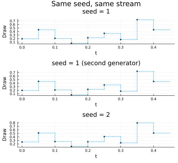
The first two panels are identical sample for sample; the third is an independent stream.
Prefer functions of their arguments
Each call written in the source is executed once per tick of its clock — the number of invocations matches the number of calls you wrote, and reusing the result does not re-invoke the function. In the example above, seeded_rand appears once per noise component and runs once per tick per component.
Determinism is still worth insisting on, for two reasons that have nothing to do with call counts:
The same call written twice should agree. Two occurrences are two invocations. If the function keeps internal state, the second occurrence sees a different value than the first, which is rarely what the equations mean. It is also what makes the two same-seed generators above coincide rather than diverge.
Runs should be reproducible. A function reading a mutable global — an RNG stream, a counter, a file position — makes the result depend on how many times it has been called so far, which couples the answer to simulation history rather than to the model.
This is why the noise sources take both a seed and the sampled time and derive their randomness from hash(t, hash(seed)) rather than from a mutable RNG: the value is a pure function of (seed, t), so it is reproducible and consistent across occurrences, while seed still gives the user control over the stream.
Apply the same rule to anything you call from a clocked equation: make the result depend only on the arguments. If a value has to change from tick to tick, feed the thing that changes — usually the sampled time — in as an argument, which is what the noise components do internally.
Functions with genuine side effects
Sometimes the point of the call is the side effect — sending a command, latching a value, talking to a device. Two things then matter.
Order between independent calls is undefined. Within a tick, if two side-effecting calls have no data dependence on each other, nothing determines which runs first. If the order matters, you must create the dependency yourself. The established way is a dependency token: have the first function return a value the later ones consume, so the data flow forces the schedule.
  # `hw_measure` latches the device's registers; its return value carries no
  # information, it exists only to order the reads that follow.
  trig@clk           = hw_measure(t@clk)
  shoulder_angle@clk = hw_shoulder(trig)
  elbow_angle@clk    = hw_elbow(trig)
Without the token, hw_shoulder and hw_elbow are independent of hw_measure as far as the compiler can tell, and could be scheduled before the call that performs the actual measurement. All three are ordinary registered functions; only the data flow between them creates the order.
Read, compute, write is a data dependency too. The same technique orders the phases of a control step: the write consumes the controller output, which consumes the reads, so the sequence is forced by construction rather than by convention.
Treat any model that relies on an incidental ordering as fragile and subject to breaking in future versions.
Talking to hardware
Hardware I/O splits into two layers:
Inside the model
A component that talks to a device or a network connection etc. looks like any other clocked component; the device access is hidden behind registered functions. On the Julia side those functions reach the driver, typically with ccall into the vendor's library:
const HIL  = "/opt/vendor/lib/libhil.so"
const CARD = Ref{Ptr{Cvoid}}(C_NULL)   # opened once at start-up

"Read one encoder channel. Takes the tick time so the call depends on the clock."
measure(_t) =
    ccall((:hil_read_encoder, HIL), Float64, (Ptr{Cvoid}, UInt32), CARD[], 0)

"Write the command, and report back the value the driver accepted."
function actuate(u)
    ccall((:hil_write_analog, HIL), Cint, (Ptr{Cvoid}, UInt32, Float64), CARD[], 0, u)
    return u
end

@register_symbolic measure(t::Real)::Real
@register_symbolic actuate(u::Real)::Real
and the Dyad component performs one tick of the loop: read, compute, write, in that order and one equation each.
component DeviceControlLoop@[input clk extends Discrete]
  "Measurement read from the device this tick"
  y = Dyad.RealOutput@[clk]()
  "Command computed this tick"
  u = Dyad.RealOutput@[clk]()
  "Command the driver reports having accepted"
  u_applied = Dyad.RealOutput@[clk]()
  "Proportional gain"
  parameter k::Real = 2.0
  "Sampled time, giving the read a clocked argument"
  sampler = DiscreteComponents.Sampler()
  clockref = BlockComponents.Sources.ContinuousClock()
  variable td::Real
relations
  connect(clockref.y, sampler.u)
  td@clk = sampler.y@clk

  y@clk         = measure(td)
  u@clk         = -k * y@clk
  u_applied@clk = actuate(u@clk)
end
The three equations read the way the tick executes. Each one consumes the previous one's result, so no dependency token is needed: actuate takes u, which was computed from y, which came from measure, and that chain is a genuine data dependency. Reach for the token pattern only when calls really are independent of one another, as two reads of different channels are.
Two details. measure takes td, the sampled time, rather than time — referring to continuous-time time inside a clocked equation is a clock error, see Connecting across the boundary. And actuate returns the value the driver accepted rather than nothing, which is worth doing because it can differ from what was requested — a driver may clamp it — so u_applied records what actually reached the device rather than what was intended.
Because this depends on a device being present, a model written this way cannot be simulated on a machine without one. Keep the plant model and the device component as separate, interchangeable implementations of the same interface, so the model can be run against a simulated plant during development and against the device when deployed.
Outside the model: the real-time loop
Driving hardware at a fixed rate is not done by the ODE solver. The controller partition is compiled to a standalone synchronous program and stepped from a loop that is responsible for the timing — see Code Generation and Deployment for how to obtain that program. The typical sequence of steps is:
Read, step, write, then sleep the remainder of the period. Sleep for what is left of the period rather than for a fixed interval, so measurement and computation time are accounted for.
A late step stretches its own period; it does not compress the next one. Recovering "lost" time by shortening subsequent periods makes a transient overrun into a burst of too-fast samples, which the controller was not designed for.
Zero the actuator and release the device on exit, including on interrupt.
Do not reset the device's counters mid-run. Zeroing a driver's counter extension has been observed to desynchronise it and produce large spurious jumps. Read the initial values once and subtract them as a software offset.
Keep allocation out of the loop so the garbage collector does not introduce latency at an arbitrary tick.
Logging data from inside the program
The natural way to record what a program did is a logging component: a clocked component whose inputs are the signals to log and whose body calls a registered function that appends one row per tick. The logging then happens inside the compiled program, alongside the hardware I/O, rather than from a loop wrapped around it — so the same model logs identically whether it runs in the simulator, through the in-process C backend, or as exported C on the target.
The component looks like any other clocked block:
component DataLogger@[input clk extends Discrete]
  "Signals to log, one column each"
  u = [Dyad.RealInput@[clk]() for i in 1:n] {^u}
  "Number of the row just written, 0 if no log is open"
  row = Dyad.RealOutput@[clk]() {^row}
  "Number of signals logged"
  structural parameter n::Integer = 1
  "File the rows are written to, opened by the driver with this name"
  structural parameter filename::String = "log.csv"
  "The inputs, padded out to the operator's fixed arity"
  variable v::Real[8]
relations
  for i in 1:n
    v[i] = u[i]
  end
  for i in n + 1:8
    v[i] = 0.0
  end
  row@clk = log_row(v[1], v[2], v[3], v[4], v[5], v[6], v[7], v[8])
end
Four design points are worth copying, because each follows from a constraint rather than from taste:
The operator has a fixed arity. A registered function has one signature — there is no variadic form, and passing an array would put an array-valued signal inside the clocked partition. So the operator takes a fixed number of columns and the component pads its unused inputs with
0.0; the driver is told how many to actually write.The filename cannot be a signal. Every value crossing a synchronous program's interface is a number, so a filename cannot be one. It is a structural parameter — a build-time value that never enters the equations — and the driver opens the file. Keep one source of truth by handing the same value to the model and to whatever opens the log.
The operator returns the row number, and that output is brought out of the component. A call whose result nothing consumes may be eliminated; returning something meaningful also lets the model react to logging state. Returning
0when no log is open means a model containing a logger still runs when nothing wants the data, which is what lets the same model be used in simulator tests.No dependency token is needed. The logged values are what the program computed this tick, so the dependency is real — the same argument as for the actuator write above.
Log the loop diagnostics alongside the signals — the achieved period and the duration of the step — so that afterwards you can tell a control problem from a missed deadline.
For the solver's own output during a simulation, TransientAnalysis takes a log_file argument; see TransientAnalysis. For tracing the compiler when code generation misbehaves, see Debug Logging.
See also
Clocks and Sampled-Data Systems — clocks, partitions and reading results
Code Generation and Deployment — compiling a controller and stepping it from a real-time loop
Measurement Noise and Corruption — the noise and quantization components built on these mechanics
Importing libraries — the Dyad
usingsyntax for Julia functionsJulia-Based Component Libraries — authoring a library with a
definitions.jl