LIBRARY

Pendulum–The "Hello World of multi-body dynamics"

This beginners tutorial will start by modeling a pendulum pivoted around the origin in the world frame. All multibody models are "grounded" in a world frame, i.e., the World component must be included exactly once in all models, at the top level.

To start, we load the required packages

using ModelingToolkit
using MultibodyComponents
using OrdinaryDiffEqDefault # Contains the ODE solver we will use
using Plots

Unless otherwise specified, the world defaults to having a gravitational field pointing in the negative direction and a gravitational acceleration of (see World for more options).

Modeling the pendulum

Our simple pendulum will initially consist of a Body (point mass) and a Revolute joint (the pivot joint). We assemble these elements, together with the World, into a Dyad component:

example component Pendulum
  world = MultibodyComponents.World()
  joint = MultibodyComponents.Revolute(n = [0, 0, 1])
  body = MultibodyComponents.Body(m = 1, r_cm = [0.5, 0, 0])
relations
  connect(world.frame_b, joint.frame_a)
  connect(joint.frame_b, body.frame_a)
end

The n argument to Revolute denotes the rotational axis of the joint, this vector must have norm(n) == 1. By default, the revolute joint is the root of the kinematic tree, i.e., the potential state of the joint will serve as the state variables for the system.

The Body is constructed by providing its mass, m, and the vector r_cm from its mounting frame, body.frame_a, to the center of mass. Since the world by default has the gravity field pointing along the negative axis, we place the center of mass along the -axis to make the pendulum swing back and forth. The body is not selected as the root of the kinematic tree, since we have a joint in this system, but if we had attached the body directly to, e.g., a spring, we could set the body to be the root and avoid having to introduce an "artificial joint", which is otherwise needed in order to have at least one component that has a potential state.

The components are connected together in the relations section using the connect function. A joint typically has two frames, frame_a and frame_b. In this example, the first frame of the joint is attached to the world frame, and the body is attached to the second frame of the joint, i.e., the joint allows the body to swing back and forth. The order of the connections is not important, but it's good practice to follow some convention, here, we start at the world and progress outwards in the kinematic tree.

With the model defined, we instantiate it in Julia and perform model check and compilation using the function multibody

@named model = Pendulum()
ssys = multibody(model)

This results in a simplified model with the minimum required variables and equations to be able to simulate the system efficiently. This step rewrites all connect statements into the appropriate equations, and removes any redundant variables and equations. To simulate the pendulum, we require two state variables, one for angle and one for angular velocity, we can see above that these state variables have indeed been chosen.

Note

The function multibody internally calls mtkcompile, and the user should thus not call mtkcompile manually for multibody systems.

MultibodyComponents.multibody Function

multibody(model)

Perform validity checks on the model, such as the presence of exactly one world component in the top level of the model, and call mtkcompile with simplification options suitable for multibody systems.

We are now ready to create an ODEProblem and simulate it. We use the Tsit5 solver from OrdinaryDiffEq.jl, and pass a dictionary for the initial conditions. We specify only initial condition for some variables, for those variables where no initial condition is specified, the default initial condition defined the model will be used.

using Main.var"##build/.dyad/stdlib/MultibodyComponents/pendulumDyadHygiene#352".pendulum # hide
defs = Dict() # We may specify the initial condition here
prob = ODEProblem(ssys, defs, (0, 3.35))

sol = solve(prob, Tsit5())
plot(sol, idxs = ssys.joint.phi, title="Pendulum")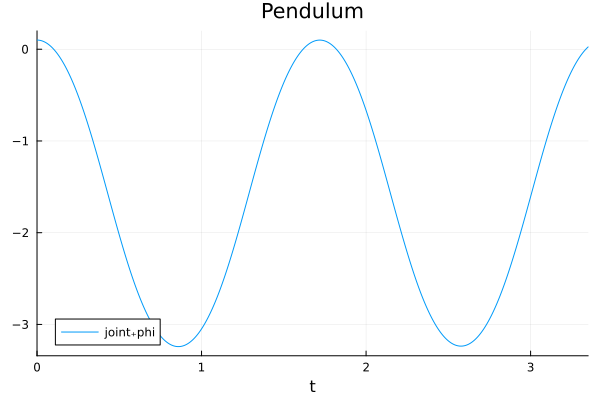

The solution sol can be plotted directly if the Plots package is loaded. The figure indicates that the pendulum swings back and forth without any damping. To add damping as well, we could add a Damper from the RotationalComponents library to the revolute joint. We do this below

3D Animation

MultibodyComponents supports automatic 3D rendering of mechanisms, we use this feature to illustrate the result of the simulation below:

using Main.var"##build/.dyad/stdlib/MultibodyComponents/pendulumDyadHygiene#352".pendulum # hide
import GLMakie
render(model, sol; filename = "pendulum_swing.gif") # Use "pendulum_swing.mp4" for a video file
HTML("<img src=\"pendulum_swing.gif\" alt=\"pendulum animation\"/>") # hide

By default, the world frame is indicated using the convention x: red, y: green, z: blue. The animation shows how the simple Body represents a point mass with inertial properties at a particular distance r_cm away from its mounting flange frame_a. The cylinder that is shown connecting the pivot point to the body is for visualization purposes only, it does not have any inertial properties. To model a more physically motivated pendulum rod, we could have used a BodyShape component, which has two mounting flanges instead of one. The BodyShape component is shown in several of the examples available in the example sections of the documentation.

Adding damping

To add damping to the pendulum such that the pendulum will eventually come to rest, we add a Damper to the revolute joint. The damping coefficient is given by d, and the damping force is proportional to the angular velocity of the joint. Every joint in MultibodyComponents exposes two rotational flanges, axis and support, to which you can attach components from the RotationalComponents library (1-dimensional components). We then connect one of the flanges of the damper to the axis flange of the joint, and the other damper flange to the support flange which is rigidly attached to the world.

example component DampedPendulum
  world = MultibodyComponents.World()
  joint = MultibodyComponents.Revolute(n = [0, 0, 1])
  body = MultibodyComponents.Body(m = 1, r_cm = [0.5, 0, 0])
  damper = RotationalComponents.Components.Damper(d = 0.3)
relations
  connect(world.frame_b, joint.frame_a)
  connect(damper.spline_b, joint.axis)
  connect(joint.support, damper.spline_a)
  connect(body.frame_a, joint.frame_b)
end

using Main.var"##build/.dyad/stdlib/MultibodyComponents/pendulumDyadHygiene#352".pendulum # hide
@named model = DampedPendulum()
ssys = multibody(model)

prob = ODEProblem(ssys, [], (0, 10))

sol = solve(prob, Tsit5())
plot(sol, idxs = ssys.joint.phi, title="Damped pendulum")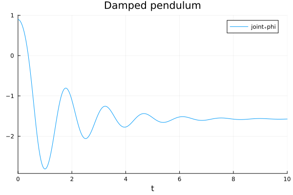

This time we see that the pendulum loses energy and eventually comes to rest at the stable equilibrium point .

using Main.var"##build/.dyad/stdlib/MultibodyComponents/pendulumDyadHygiene#352".pendulum # hide
render(model, sol; filename = "pendulum_damped.gif")
HTML("<img src=\"pendulum_damped.gif\" alt=\"damped pendulum animation\"/>") # hide

A linear pendulum?

When we think of a pendulum, we typically think of a rotary pendulum that is rotating around a pivot point like in the examples above. A mass suspended in a spring can be though of as a linear pendulum (often referred to as a harmonic oscillator rather than a pendulum), and we show here how we can construct a model of such a device. This time around, we make use of a Prismatic joint rather than a Revolute joint. A prismatic joint has one positional degree of freedom, compared to the single rotational degree of freedom for the revolute joint.

example component LinearPendulum
  world = MultibodyComponents.World()
  body_0 = MultibodyComponents.Body(m = 1, r_cm = [0, 0, 0])
  damper = TranslationalComponents.Components.Damper(d = 1)
  spring = TranslationalComponents.Components.Spring(c = 10)
  joint = MultibodyComponents.Prismatic(n = [0, 1, 0])
relations
  connect(world.frame_b, joint.frame_a)
  connect(damper.flange_b, spring.flange_b, joint.axis)
  connect(joint.support, damper.flange_a, spring.flange_a)
  connect(body_0.frame_a, joint.frame_b)
end

using Main.var"##build/.dyad/stdlib/MultibodyComponents/pendulumDyadHygiene#352".pendulum # hide
@named model = LinearPendulum()
ssys = multibody(model)

prob = ODEProblem(ssys, [ssys.joint.s => 0, ssys.joint.v => 0], (0, 10))

sol = solve(prob, Tsit5())
Plots.plot(sol, idxs = ssys.joint.s, title="Mass-spring-damper system")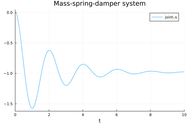

As is hopefully evident from the little code snippet above, this linear pendulum model has a lot in common with the rotary pendulum. In this example, we connected both the spring and a damper to the same axis flange in the joint. This time, the components came from the TranslationalComponents library rather than RotationalComponents. Also here is the joint equipped with the flanges support and axis needed to connect the translational components.

using Main.var"##build/.dyad/stdlib/MultibodyComponents/pendulumDyadHygiene#352".pendulum # hide
render(model, sol; filename = "linear_pend.gif", framerate=24)
HTML("<img src=\"linear_pend.gif\" alt=\"linear pendulum animation\"/>") # hide

Why do we need a joint?

In the example above, we introduced a prismatic joint to model the oscillating motion of the mass-spring system. In reality, we can suspend a mass in a spring without any joint, so why do we need one here? The answer is that we do not, in fact, need the joint, but if we connect the spring directly to the world, we need to make the body (mass) the root object of the kinematic tree instead:

example component MassSpring
  world = MultibodyComponents.World()
  multibody_spring = MultibodyComponents.Spring(c = 10)
  root_body = MultibodyComponents.Body(m = 1, r_cm = [0, 1, 0], orientation_state = MultibodyComponents.OrientationState.Quaternion())
relations
  connect(world.frame_b, multibody_spring.frame_a)
  connect(root_body.frame_a, multibody_spring.frame_b)
end

using Main.var"##build/.dyad/stdlib/MultibodyComponents/pendulumDyadHygiene#352".pendulum # hide
@named model = MassSpring()
ssys = multibody(model)

defs = Dict(collect(ssys.root_body.r_0) .=> [0, 1e-3, 0]) # The spring has a singularity at zero length, so we start some distance away

prob = ODEProblem(ssys, defs, (0, 10))

sol = solve(prob, Tsit5())
plot(sol, idxs = ssys.multibody_spring.r_rel_0[2], title="Mass-spring system without joint")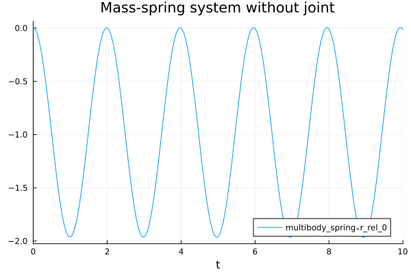

Here, we used a Spring instead of connecting a TranslationalComponents.Components.Spring to a joint. The TranslationalComponents.Components.Spring, alongside other 1-dimensional mechanical components, is a 1-dimensional object, whereas multibody components are 3-dimensional objects. In this latter example, the state will be 13 dimensional, 3 positional DOFs and their velocities plus a 4-dimensional quaternion and three angular velocities. This is in contrast to the earlier pendulum with the joint that had a 2-dimensional state, a single position coordinate and its velocity.

Internally, the Spring contains a TranslationalComponents.Components.Spring, attached between two flanges, so we could actually add a damper to the system as well:

example component MassSpringDamper
  world = MultibodyComponents.World()
  multibody_spring = MultibodyComponents.Spring(c = 10)
  root_body = MultibodyComponents.Body(m = 1, r_cm = [0, 1, 0], orientation_state = MultibodyComponents.OrientationState.Quaternion())
  damper = TranslationalComponents.Components.Damper(d = 1)
relations
  connect(world.frame_b, multibody_spring.frame_a)
  connect(root_body.frame_a, multibody_spring.frame_b)
  connect(multibody_spring.spring1d.flange_a, damper.flange_a)
  connect(multibody_spring.spring1d.flange_b, damper.flange_b)
end

using Main.var"##build/.dyad/stdlib/MultibodyComponents/pendulumDyadHygiene#352".pendulum # hide
@named model = MassSpringDamper()
ssys = multibody(model)
prob = ODEProblem(ssys, defs, (0, 10))

sol = solve(prob, Rodas4(), u0 = prob.u0 .+ 1e-5 .* randn.())
plot(sol, idxs = ssys.multibody_spring.r_rel_0[2], title="Mass-spring-damper without joint")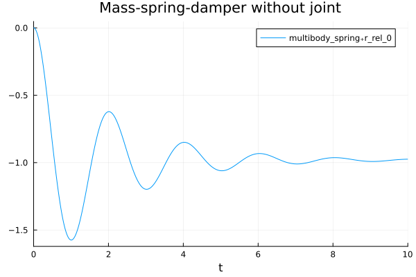

The figure above should look identical to the simulation of the mass-spring-damper further above.

Going 3D

The systems we have modeled so far have all been planar mechanisms. We now extend this to a 3-dimensional system, the Furuta pendulum.

This pendulum, sometimes referred to as a rotary pendulum, has two joints, one in the "shoulder", which is typically configured to rotate around the gravitational axis, and one in the "elbow", which is typically configured to rotate around the axis of the upper arm. The upper arm is attached to the shoulder joint, and the lower arm is attached to the elbow joint. The tip of the pendulum is attached to the lower arm.

example component FurutaPendulum
  world = MultibodyComponents.World()
  shoulder_joint = MultibodyComponents.Revolute(n = [0, 1, 0])
  elbow_joint = MultibodyComponents.Revolute(n = [0, 0, 1], phi = initial 0.1)
  upper_arm = MultibodyComponents.BodyShape(m = 0.1, r = [0, 0, 0.6], radius = 0.04)
  lower_arm = MultibodyComponents.BodyShape(m = 0.1, r = [0, 0.6, 0], radius = 0.04)
  tip = MultibodyComponents.Body(m = 0.3)
  damper1 = RotationalComponents.Components.Damper(d = 0.07)
  damper2 = RotationalComponents.Components.Damper(d = 0.07)
relations
  connect(world.frame_b, shoulder_joint.frame_a)
  connect(shoulder_joint.frame_b, upper_arm.frame_a)
  connect(upper_arm.frame_b, elbow_joint.frame_a)
  connect(elbow_joint.frame_b, lower_arm.frame_a)
  connect(lower_arm.frame_b, tip.frame_a)

  connect(shoulder_joint.axis, damper1.spline_a)
  connect(shoulder_joint.support, damper1.spline_b)

  connect(elbow_joint.axis, damper2.spline_a)
  connect(elbow_joint.support, damper2.spline_b)
end

using Main.var"##build/.dyad/stdlib/MultibodyComponents/pendulumDyadHygiene#352".pendulum # hide
@named model = FurutaPendulum()
ssys = multibody(model)

prob = ODEProblem(ssys, [ssys.shoulder_joint.phi => 0.0, ssys.elbow_joint.phi => 0.1], (0, 10))
sol = solve(prob, Tsit5())
plot(sol, layout=4)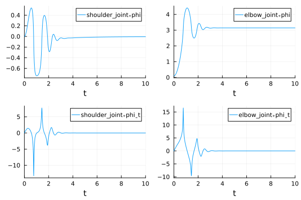

In the animation below, we visualize the path that the origin of the pendulum tip traces by providing the tip frame in a vector of frames passed to traces

using Main.var"##build/.dyad/stdlib/MultibodyComponents/pendulumDyadHygiene#352".pendulum # hide
render(model, sol, filename = "furuta.gif", traces=[ssys.tip.frame_a])
HTML("<img src=\"furuta.gif\" alt=\"Furuta pendulum animation\"/>") # hide

Orientations and directions

Let's break down how to think about directions and orientations when building 3D mechanisms. In the example above, we started with the shoulder joint, this joint rotated around the gravitational axis, n = [0, 1, 0]. When this joint is positioned in joint coordinate shoulder_joint.phi = 0, its frame_a and frame_b will coincide. When the joint rotates, frame_b will rotate around the axis n of frame_a. The frame_a of the joint is attached to the world, so the joint will rotate around the world's y-axis:

using Main.var"##build/.dyad/stdlib/MultibodyComponents/pendulumDyadHygiene#352".pendulum # hide
get_rot(sol, ssys.shoulder_joint.frame_b, 0)

we see that at time  , we have no rotation of frame_b around the axis of the world (frames are always resolved in the world frame), but a second into the simulation, we have:

using Main.var"##build/.dyad/stdlib/MultibodyComponents/pendulumDyadHygiene#352".pendulum # hide
R1 = get_rot(sol, ssys.shoulder_joint.frame_b, 1)

Here, the frame_b has rotated around the axis of the world (if you are not familiar with rotation matrices, we can ask for the rotation axis and angle)

using Main.var"##build/.dyad/stdlib/MultibodyComponents/pendulumDyadHygiene#352".pendulum # hide
using MultibodyComponents.Rotations
rotation_axis(R1), rotation_angle(R1)

This rotation axis and angle should correspond to the joint coordinate (the orientation described by an axis and an angle is invariant to a multiplication of both by -1)

using Main.var"##build/.dyad/stdlib/MultibodyComponents/pendulumDyadHygiene#352".pendulum # hide
sol(1, idxs=ssys.shoulder_joint.phi)

Convention

The convention used in get_rot is to return the rotation matrix that rotates a coordinate from the local frame to the world frame,  .

Here, we made use of the function get_rot, we will now make use of also get_trans and get_frame.

The next body is the upper arm. This body has an extent of 0.6 in the direction, as measured in its local frame_a

using Main.var"##build/.dyad/stdlib/MultibodyComponents/pendulumDyadHygiene#352".pendulum # hide
get_trans(sol, ssys.upper_arm.frame_b, 0)

One second into the simulation, the upper arm has rotated around the axis of the world

using Main.var"##build/.dyad/stdlib/MultibodyComponents/pendulumDyadHygiene#352".pendulum # hide
rb1 = get_trans(sol, ssys.upper_arm.frame_b, 1)

If we look at the variable ssys.upper_arm.r, we do not see this rotation!

using Main.var"##build/.dyad/stdlib/MultibodyComponents/pendulumDyadHygiene#352".pendulum # hide
arm_r = sol(1, idxs=ssys.upper_arm.r)

The reason is that this variable is resolved in the local frame_a and not in the world frame. To transform this variable to the world frame, we may multiply with the rotation matrix of frame_a which is always resolved in the world frame:

using Main.var"##build/.dyad/stdlib/MultibodyComponents/pendulumDyadHygiene#352".pendulum # hide
get_rot(sol, ssys.upper_arm.frame_a, 1)*arm_r

We now get the same result has when we asked for the translation vector of frame_b above.

using Main.var"##build/.dyad/stdlib/MultibodyComponents/pendulumDyadHygiene#352".pendulum # hide
using Test # hide
get_rot(sol, ssys.upper_arm.frame_a, 1)*arm_r ≈ rb1 # hide
nothing # hide

Slightly more formally, let denote the rotation matrix that rotates a vector expressed in a frame into one that is expressed in frame , i.e.,  . We have then just performed the transformation  , where denotes the world frame, and denotes body.frame_a.

The next joint, the elbow joint, has the rotational axis n = [0, 0, 1]. This indicates that the joint rotates around the -axis of its frame_a. Since the upper arm was oriented along the direction, the joint is rotating around the axis that coincides with the upper arm.

The lower arm is finally having an extent along the -axis. At the final time when the pendulum motion has been fully damped, we see that the second frame of this body ends up with an -coordinate of -0.6:

using Main.var"##build/.dyad/stdlib/MultibodyComponents/pendulumDyadHygiene#352".pendulum # hide
get_trans(sol, ssys.lower_arm.frame_b, 12)

If we rotate the vector of extent of the lower arm to the world frame, we indeed see that the only coordinate that is nonzero is the coordinate:

using Main.var"##build/.dyad/stdlib/MultibodyComponents/pendulumDyadHygiene#352".pendulum # hide
get_rot(sol, ssys.lower_arm.frame_a, 12)*sol(12, idxs=ssys.lower_arm.r)

The reason that the latter vector differs from get_trans(sol, ssys.lower_arm.frame_b, 12) above is that get_trans(sol, ssys.lower_arm.frame_b, 12) has been translated as well. To both translate and rotate ssys.lower_arm.r into the world frame, we must use the full transformation matrix  :

using Main.var"##build/.dyad/stdlib/MultibodyComponents/pendulumDyadHygiene#352".pendulum # hide
r_A = sol(12, idxs=ssys.lower_arm.r)
r_A = [r_A; 1] # Homogeneous coordinates

get_frame(sol, ssys.lower_arm.frame_a, 12)*r_A

the vector is now coinciding with get_trans(sol, ssys.lower_arm.frame_b, 12).

Control-design example: Pendulum on cart

We will now demonstrate a complete workflow including

• Modeling

• Linearization

• Control design

We will continue the pendulum theme and design an inverted pendulum on cart. The cart is modeled as a BodyShape with specified mass, and shape = "box" to render it as a box in animations. The cart is moving along the -axis by means of a Prismatic joint, and the pendulum is attached to the cart by means of a Revolute joint. The pendulum is a BodyCylinder with a diameter of 0.015, the mass and inertia properties are automatically computed using the geometrical dimensions and the density (which defaults to that of steel). A force is applied to the cart by means of a TranslationalComponents.Sources.Force component.

We start by putting the model together and control it in open loop using a simple periodic input signal:

component Cartpole
  u = RealInput()
  fixed = MultibodyComponents.Fixed()
  cart = MultibodyComponents.BodyShape(m = 1, r = [0.2, 0, 0], shape = "box", width = 0.1, height = 0.1, color = [0.2, 0.2, 0.2, 1])
  mounting_point = MultibodyComponents.FixedTranslation(r = [0.1, 0, 0])
  prismatic = MultibodyComponents.Prismatic(n = [1, 0, 0], statePriority = 100, color = [0.5, 0.5, 0.5, 1])
  revolute = MultibodyComponents.Revolute(n = [0, 0, 1], statePriority = 100)
  pendulum = MultibodyComponents.BodyCylinder(r = [0, 0.5, 0], diameter = 0.015, color = [0.5, 0.5, 0.5, 1])
  motor = TranslationalComponents.Sources.Force()
  tip = MultibodyComponents.Body(m = 0.05)
  variable x::Length
  variable v::Velocity
  variable phi::Angle
  variable w::AngularVelocity
relations
  connect(fixed.frame_b, prismatic.frame_a)
  connect(prismatic.frame_b, cart.frame_a, mounting_point.frame_a)
  connect(mounting_point.frame_b, revolute.frame_a)
  connect(revolute.frame_b, pendulum.frame_a)
  connect(pendulum.frame_b, tip.frame_a)
  connect(motor.flange_a, prismatic.support)
  connect(motor.flange_b, prismatic.axis)
  connect(u, motor.f)
  x = prismatic.s
  v = prismatic.v
  phi = revolute.phi
  w = revolute.w
end

example component CartWithInput
  world = MultibodyComponents.World()
  cartpole = Cartpole()
  input = BlockComponents.Sources.Cosine(frequency = 1, amplitude = 1)
relations
  connect(input.y, cartpole.u)
end

using Main.var"##build/.dyad/stdlib/MultibodyComponents/pendulumDyadHygiene#352".pendulum # hide
@named model = CartWithInput()
ssys = multibody(model)
prob = ODEProblem(ssys, [ssys.cartpole.prismatic.s => 0.0, ssys.cartpole.prismatic.v => 0.0, ssys.cartpole.revolute.phi => 0.1], (0, 10))
sol = solve(prob, Tsit5())
plot(sol, layout=4)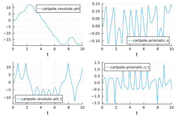

As usual, we render the simulation in 3D to get a better feel for the system:

using Main.var"##build/.dyad/stdlib/MultibodyComponents/pendulumDyadHygiene#352".pendulum # hide
render(model, sol, filename = "cartpole.gif", traces=[ssys.cartpole.pendulum.frame_b])
HTML("<img src=\"cartpole.gif\" alt=\"cartpole animation\"/>") # hide

Adding feedback

We will attempt to stabilize the pendulum in the upright position by using feedback control. To design the controller, we linearize the model in the upward equilibrium position and design an infinite-horizon LQR controller using ControlSystems.jl. We then connect the controller to the motor on the cart. See also RobustAndOptimalControl.jl: Control design for a pendulum on a cart for a similar example with more detail on the control design.

Linearization

We start by linearizing the model in the upward equilibrium position using the function ModelingToolkit.linearize. Since all multibody models must contain a world, we wrap the cartpole in a component that adds the world as well as exposes the interesting outputs as top-level variables:

component OpenLoopCartpole
  world = MultibodyComponents.World()
  cartpole = Cartpole()
  variable x::Length
  variable v::Velocity
  variable phi::Angle
  variable w::AngularVelocity
relations
  x = cartpole.x
  v = cartpole.v
  phi = cartpole.phi
  w = cartpole.w
end

using LinearAlgebra
@named cp = OpenLoopCartpole()
ncp = ModelingToolkit.toggle_namespacing(cp, false) # Address variables via a non-namespaced view
inputs = [ncp.cartpole.u] # Input to the linearized system
outputs = [ncp.x, ncp.phi, ncp.v, ncp.w] # These are the outputs of the linearized system
op = Dict([ # Operating point to linearize in
    ncp.cartpole.u            => 0
    ncp.cartpole.prismatic.s  => 0
    ncp.cartpole.prismatic.v  => 0
    ncp.cartpole.revolute.phi => 0 # Pendulum pointing upwards
    ncp.cartpole.revolute.w   => 0
])
matrices, simplified_sys = ModelingToolkit.linearize(cp, inputs, outputs; op, MultibodyComponents.linsys...)
matrices

(A = [0.0 0.0 0.0 1.0; 0.0 0.0 1.0 0.0; 4.474102070258826 0.0 0.0 0.0; 39.68350716589239 -0.0 -0.0 -0.0], B = [0.0; 0.0; 0.8415814526118871; 2.338595575436011;;], C = [0.0 1.0 0.0 0.0; 1.0 0.0 0.0 0.0; 0.0 0.0 1.0 0.0; 0.0 0.0 0.0 1.0], D = [0.0; 0.0; 0.0; 0.0;;])

This gives us the matrices in a linearized statespace representation of the system. To make these easier to work with, we load the control packages and call named_ss instead of linearize to get a named statespace object instead:

using ControlSystemsMTK
lsys = named_ss(cp, inputs, outputs; op, MultibodyComponents.linsys...) # identical to linearize, but packages the resulting matrices in a named statespace object for convenience

cp: NamedControlSystemsBase.StateSpace{ControlSystemsBase.Continuous, Float64}
A = 
  0.0                 0.0   0.0   1.0
  0.0                 0.0   1.0   0.0
  4.474102070258826   0.0   0.0   0.0
 39.68350716589239   -0.0  -0.0  -0.0
B = 
 0.0
 0.0
 0.8415814526118871
 2.338595575436011
C = 
 0.0  1.0  0.0  0.0
 1.0  0.0  0.0  0.0
 0.0  0.0  1.0  0.0
 0.0  0.0  0.0  1.0
D = 
 0.0
 0.0
 0.0
 0.0

Continuous-time state-space model
With state  names: cartpole₊revolute₊phi(t) cartpole₊prismatic₊s(t) cartpole₊prismatic₊v(t) cartpole₊revolute₊w(t)
     input  names: cartpole₊u(t)
     output names: x(t) phi(t) v(t) w(t)
Operating point: x = [0.0, 0.0, 0.0, 0.0], u = [0.0]

LQR and LQG Control design

With a linear statespace object in hand, we can proceed to design an LQR or LQG controller. We will design both an LQR and an LQG controller in order to demonstrate two possible workflows.

The LQR controller is designed using the function ControlSystemsBase.lqr, and it takes the two cost matrices Q1 and Q2 penalizing state deviation and control action respectively. The LQG controller is designed using RobustAndOptimalControl.LQGProblem, and this function additionally takes the covariance matrices r1, R2 for a Kalman filter. Before we call LQGProblem we partition the linearized system into an ExtendedStateSpace object, this indicates which inputs of the system are available for control and which are considered disturbances, and which outputs of the system are available for measurement. In this case, we assume that we have access to the cart position and the pendulum angle, and we control the cart position. The remaining two outputs are still important for the performance, but we cannot measure them and will rely on the Kalman filter to estimate them. When we call extended_controller we get a linear system that represents the combined state estimator and state feedback controller. This linear system is embedded in a BlockComponents.Continuous.StateSpace component, whose matrices are provided as parameters when the model is instantiated.

Since the function lqr operates on the state vector, and we have access to the specified output vector, we make use of the system matrix to reformulate the problem in terms of the outputs. This relies on the matrix being full rank, which is the case here since our outputs include a complete state realization of the system. This is of no concern when using the LQGProblem structure since we penalize outputs rather than the state in this case.

To make the simulation interesting, we make a change in the reference position of the cart after a few seconds.

using DyadControlSystems
C = lsys.C
Q1 = Diagonal([10, 10, 10, 1]) # LQR cost matrices
Q2 = Diagonal([0.1])

R1 = lsys.B*Diagonal([1])*lsys.B' # Kalman covariance matrices
R2 = Diagonal([0.01, 0.01])
Pn = lsys[[:x, :phi], :]    # Named system with only cart position and pendulum angle measurable

lqg = LQGProblem(ss(Pn), Q1, Q2, R1, R2)
Lmat = lqr(lsys, C'Q1*C, Q2)/C # Alternatively, compute LQR feedback gain. The multiplication by the C matrix is to handle the difference between state and output

# Compute a static gain compensation
z = [:x] # The output for which we want to have unit static gain
Ce, cl = extended_controller(lqg, z = DyadControlSystems.RobustAndOptimalControl.names2indices(z, Pn.y))
dc_gain_compensation = inv((Pn[:x, :].C*dcgain(cl)')[]) # Multiplier that makes the static gain from references to cart position unity
Cess = ss(Ce) # The combined estimator and state feedback controller as a plain statespace system

ControlSystemsBase.StateSpace{ControlSystemsBase.Continuous, Float64}
A = 
  -12.930634154506967   -1.3387562007039728   0.0                  1.0
   -1.3387562007039728  -3.413865019111676    1.0                  0.0
  -76.51243982409572     1.692443259300628   12.885729396459764  -12.6546951543445
 -238.65398847251583    12.734481876779745   35.80700318347404   -35.165002751182975
B = 
   0.0                 0.0                  0.0                 0.0                 1.3387562007039728  12.930634154506967
   0.0                 0.0                  0.0                 0.0                 3.413865019111676    1.3387562007039728
  69.7567161558541    -8.415814526119496  -12.885729396459764  12.6546951543445     6.723371266818868   11.229825738500457
 193.84071173709452  -23.38595575436185   -35.80700318347404   35.165002751182975  10.651473877582104   84.49678390131369
C = 
 -82.8876586328761  10.000000000000743  15.311327687258679  -15.036803763997016
D = 
 82.8876586328761  -10.000000000000743  -15.311327687258679  15.036803763997016  0.0  0.0

Continuous-time state-space model

example component CartWithFeedback
  world = MultibodyComponents.World()
  cartpole = Cartpole()
  reference = BlockComponents.Sources.Step(start_time = 5, height = 0.5)
  controller = BlockComponents.Continuous.StateSpace(nx = 4, nu = 6, ny = 1, A = A, B = B, C = C, D = D)
  control_saturation = BlockComponents.Nonlinear.Limiter(y_max = 10)
  parameter A::Real[4, 4] = fill(0, 4, 4)
  parameter B::Real[4, 6] = fill(0, 4, 6)
  parameter C::Real[1, 4] = fill(0, 1, 4)
  parameter D::Real[1, 6] = fill(0, 1, 6)
  parameter dc_gain_compensation::Real = 1
  variable yc::Real[1]
relations
  controller.u = [0, dc_gain_compensation * reference.y, 0, 0, cartpole.x, cartpole.phi]
  yc = controller.y
  control_saturation.u = yc[1]
  connect(control_saturation.y, cartpole.u)
end

using Main.var"##build/.dyad/stdlib/MultibodyComponents/pendulumDyadHygiene#352".pendulum # hide
@named model = CartWithFeedback(A = Cess.A, B = Cess.B, C = Cess.C, D = Cess.D, dc_gain_compensation)
ssys = multibody(model)
prob = ODEProblem(ssys, [ssys.cartpole.prismatic.s => 0.1, ssys.cartpole.prismatic.v => 0.0, ssys.cartpole.revolute.phi => 0.35, ssys.cartpole.revolute.w => 0.0], (0, 12))
sol = solve(prob, Tsit5())
cp = ssys.cartpole
plot(sol, idxs=[cp.prismatic.s, cp.revolute.phi, cp.u], layout=3)
plot!(sol, idxs=ssys.reference.y, sp=1, l=(:black, :dash), legend=:bottomright)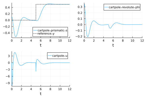

using Main.var"##build/.dyad/stdlib/MultibodyComponents/pendulumDyadHygiene#352".pendulum # hide
render(model, sol, filename = "inverted_cartpole.gif", x=1, z=1)
HTML("<img src=\"inverted_cartpole.gif\" alt=\"inverted cartpole animation\"/>") # hide

Swing up

Below, we add also an energy-based swing-up controller. For more details on this kind of swing-up controller, see Part 7: Control of rotary pendulum using Julia: Swing up control (YouTube)

The controller is based on the total energy of the pendulum. Every Body provides the variables KE and PE with the kinetic and potential energy of the body, and we sum these variables for the pendulum body and the tip mass to obtain the total energy. Since the cart is moving, we express the energy in the reference frame of the cart by means of a Galilean transformation, subtracting the energy contribution due to the cart velocity. The controller pumps energy into the pendulum until it slightly exceeds the energy Er at the upright equilibrium, the margin E_margin makes the pendulum pass the upright position with a small velocity such that the stabilizing controller can catch it. During the swing-up phase, a weak feedback from the cart position and velocity keeps the cart close to the origin.

example component CartWithSwingup
  world = MultibodyComponents.World()
  cartpole = Cartpole()
  control_saturation = BlockComponents.Nonlinear.Limiter(y_max = 12)
  "LQR feedback gain of the stabilizing controller"
  parameter L::Real[4]
  "Total energy of the pendulum at the upright equilibrium"
  parameter Er::Real
  "Energy pumped in excess of the upright equilibrium energy"
  parameter E_margin::Real = 0.4
  "Feedback gain of the energy-based swing-up controller"
  parameter k_swing::Real = 100
  "Cart position feedback gain during swing-up"
  parameter k_x::Real = 2
  "Cart velocity feedback gain during swing-up"
  parameter k_v::Real = 4
  "Pendulum angle threshold below which the stabilizing controller is active"
  parameter phi_switch::Real = 0.4
  "Pendulum angle, normalized to be zero when the pendulum points up"
  variable phi::Angle
  "Pendulum angular velocity"
  variable w::AngularVelocity
  "Total energy of the pendulum, expressed in the reference frame of the cart"
  variable E::Real
  "Swing-up control signal"
  variable u_swing::Real
  "Stabilizing control signal"
  variable u_stab::Real
  "Indicator that equals one when the stabilizing controller is active"
  variable switching_condition::Real
relations
  phi = mod(cartpole.phi + pi, 2 * pi) - pi
  w = cartpole.w
  # The energy of the pendulum is expressed in the reference frame of the cart by
  # subtracting the contribution of the cart velocity (Galilean transformation)
  E = cartpole.pendulum.body.KE + cartpole.pendulum.body.PE + cartpole.tip.KE + cartpole.tip.PE - cartpole.v * (cartpole.pendulum.body.m * cartpole.pendulum.body.v_cm_0[1] + cartpole.tip.m * cartpole.tip.v_cm_0[1]) + 0.5 * (cartpole.pendulum.body.m + cartpole.tip.m) * cartpole.v ^ 2
  u_swing = k_swing * (E - (Er + E_margin)) * sign(w * cos(phi - pi)) - k_x * cartpole.x - k_v * cartpole.v
  u_stab = -(L[1] * cartpole.x + L[2] * phi + L[3] * cartpole.v + L[4] * cartpole.w)
  switching_condition = ifelse(abs(phi) < phi_switch, 1, 0)
  control_saturation.u = ifelse(switching_condition > 0.5, u_stab, u_swing)
  connect(control_saturation.y, cartpole.u)
end

The reference energy Er, the total energy of the pendulum at the upright equilibrium, is computed from the model rather than being hardcoded. We build a problem with the pendulum resting in the upright position and read the value of the energy variable E:

@named model = CartWithSwingup(L = vec(Lmat), Er = 0)
ssys = multibody(model)
cp = ssys.cartpole

prob0 = ODEProblem(ssys, [cp.prismatic.s => 0.0, cp.prismatic.v => 0.0, cp.revolute.phi => 0.0, cp.revolute.w => 0.0], (0, 5))
Er = prob0[ssys.E]

1.9131576734573559

using Main.var"##build/.dyad/stdlib/MultibodyComponents/pendulumDyadHygiene#352".pendulum # hide
prob = ODEProblem(ssys, [cp.prismatic.s => 0.0, cp.prismatic.v => 0.0, cp.revolute.phi => 0.99pi, cp.revolute.w => 0.0, ssys.Er => Er], (0, 5))
sol = solve(prob, Tsit5(), dt = 1e-2, adaptive=false)
plot(sol, idxs=[cp.prismatic.s, cp.revolute.phi, cp.u, ssys.E], layout=4)
hline!([0, 2pi], sp=2, l=(:black, :dash), primary=false)
plot!(sol, idxs=[ssys.switching_condition], sp=2)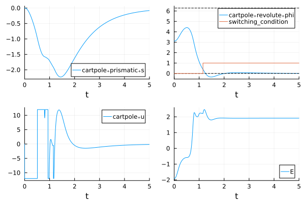

using Main.var"##build/.dyad/stdlib/MultibodyComponents/pendulumDyadHygiene#352".pendulum # hide
using Test # hide
phi_end = sol(sol.t[end], idxs = cp.revolute.phi) # hide
@test abs(mod(phi_end + pi, 2pi) - pi) < 0.1 # hide
nothing # hide

using Main.var"##build/.dyad/stdlib/MultibodyComponents/pendulumDyadHygiene#352".pendulum # hide
render(model, sol, filename = "swingup.gif", x=2, z=2)
HTML("<img src=\"swingup.gif\" alt=\"cartpole swingup animation\"/>") # hide