TUTORIAL

Measurement Noise and Corruption

Measurement noise is practically always present in signals originating from real-world sensors. In a sampled-data system, analyzing the influence of measurement noise using simulation is relatively straightforward. Below, we add Gaussian white noise to the speed sensor signal in the DC-motor example from DC Motor with PI Controller. The noise is added using the NormalNoise component together with an Add block.

The NormalNoise component generates Gaussian noise with configurable mean mu and standard deviation sigma. It has a single output connector y. To add noise to a signal, connect both the signal and the noise output to an Add block.

Example: Noise

This example is a continuation of the DC-motor example from DC Motor with PI Controller. We add Gaussian white noise with   to the speed sensor signal. Download as a Dyad projectNOISE.zipOpen in Dyad Studio›

"""
DC motor speed control with noisy speed measurement.
Gaussian noise is added to the sampled speed signal before it reaches the controller.
"""
test component NoisyDCMotor
  "Electrical components"
  ground = ElectricalComponents.Analog.Basic.Ground()
  source = ElectricalComponents.Analog.Sources.VoltageSource()
  R1 = ElectricalComponents.Analog.Basic.Resistor(R = 0.5)
  L1 = ElectricalComponents.Analog.Basic.Inductor(L = 4.5e-3)
  emf = ElectricalComponents.Analog.Basic.RotationalEMF(k = 0.5)
  "Mechanical components"
  fixed = RotationalComponents.Components.Fixed()
  inertia = RotationalComponents.Components.Inertia(J = 0.02)
  friction = RotationalComponents.Components.Damper(d = 0.01)
  speed_sensor = RotationalComponents.Sensors.VelocitySensor()
  load = RotationalComponents.Sources.TorqueSource()
  "Signal sources"
  ref = BlockComponents.Sources.Step(height = 1, start_time = 0)
  load_step = BlockComponents.Sources.Step(height = -0.3, start_time = 1.3)
  "Discrete-time components"
  sampler = DiscreteComponents.Sampler()
  "The continuous reference must be sampled before entering the discrete partition"
  ref_sampler = DiscreteComponents.Sampler()
  clock = DiscreteComponents.PeriodicClock(dt = 0.002)
  noise = DiscreteComponents.NormalNoise(sigma = 0.1)
  add_noise = BlockComponents.Math.Add()
  pi_controller = DiscreteComponents.DiscretePIDStandard(K = 1, Ti = 0.035, y_max = 10, with_D = false)
  zoh = DiscreteComponents.ZeroOrderHold()
relations
  initial inertia.w = 0
  initial inertia.phi = 0
  initial L1.i = 0
  # Mechanical connections
  connect(fixed.spline, emf.housing, friction.spline_b)
  connect(emf.rotor, friction.spline_a, inertia.spline_a)
  connect(inertia.spline_b, load.spline)
  connect(inertia.spline_b, speed_sensor.spline)
  connect(load.support, fixed.spline)
  connect(load_step.y, load.tau)
  # Controller connections
  connect(ref.y, ref_sampler.u)
  connect(ref_sampler.y, pi_controller.u_s)
  connect(speed_sensor.w, sampler.u)
  connect(sampler.y, add_noise.u1, clock.y)
  connect(noise.y, add_noise.u2)
  connect(add_noise.y, pi_controller.u_m)
  connect(pi_controller.y, zoh.u)
  connect(zoh.y, source.V)
  # Electrical connections
  connect(source.p, R1.p)
  connect(R1.n, L1.p)
  connect(L1.n, emf.p)
  connect(emf.n, source.n, ground.g)
end

analysis NoisyDCMotorAnalysis
  extends TransientAnalysis(stop = 2.0)
  model = NoisyDCMotor()
end

using Plots
result = NoisyDCMotorAnalysis()
using DyadInterface
model = artifacts(result, :SimplifiedSystem)
figy = plot(result; idxs = [model.add_noise.y, model.inertia.w], ylabel = "Angular Vel. [rad/s]",
    labels = ["Measured speed" "Actual speed"], legend = :bottomleft)
figu = plot(result; idxs = model.source.V, label = "Control signal [V]")
plot(figy, figu, layout = (2, 1), plot_title = "DC Motor with Noisy Speed Measurement")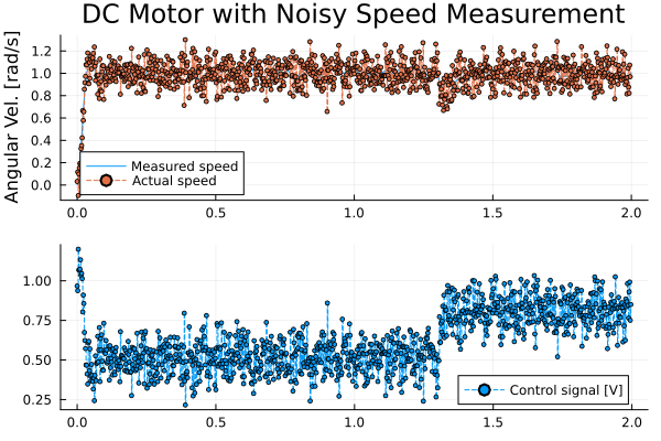

Noise filtering

You may use the following discrete-time filter components from DiscreteComponents to reduce noise:

• ExponentialFilter: First-order exponential filtering using y@clk = (1 - a) * y@(clk-1) + a * u@clk, where a is the filter coefficient. A small value of a implies stronger filtering.

• MovingAverageFilter: Moving average filtering according to y@clk = (1/N) * sum(u@(clk-i) for i=0:N-1), where N is the number of samples to average over.

Colored noise

Colored noise can be achieved by filtering white noise through a filter with the desired spectrum. For example, connect a NormalNoise to an ExponentialFilter to produce low-pass filtered noise.

Internal details

Internally, a random number generator from StableRNGs.jl is used to produce reproducible streams of random numbers. Each draw of a random number is seeded by hash(t, hash(seed)), where seed is a parameter in the noise source component, and t is the current simulation time. This ensures that:

1. The user can alter the stream of random numbers with seed.

2. Multiple calls to the random number generator at the same time step all return the same number.

Quantization

A signal may be quantized to a fixed number of levels (e.g., 8-bit) using the Quantization component. This may be used to simulate, e.g., the quantization that occurs in an AD converter. Below, we have a simple example where a sine wave is quantized to 2 bits (4 levels), limited between -1 and 1:

"""
Demonstrates quantization of a sine wave signal to 2 bits (4 levels).
"""
test component QuantizationDemo
  input_signal = BlockComponents.Sources.Sine(amplitude = 1.5, frequency = 1) {^input_signal}
  sampler = DiscreteComponents.Sampler() {^sampler}
  clock = DiscreteComponents.PeriodicClock(dt = 0.1) {^clock}
  quant = DiscreteComponents.Quantization(bits = 2, y_min = -1, y_max = 1) {^quant}
relations
  connect(input_signal.y, sampler.u) {^id4}
  connect(sampler.y, quant.u, clock.y) {^id5}
metadata {
  "_links": {
    "input_signal": {
      "Dyad": {
        "placement": {
          "diagram": {"iconName": "default", "x1": 20, "y1": 20, "x2": 220, "y2": 220, "rot": 0}
        },
        "tags": []
      }
    },
    "sampler": {
      "Dyad": {
        "placement": {
          "diagram": {"iconName": "default", "x1": 270, "y1": 20, "x2": 470, "y2": 220, "rot": 0}
        },
        "tags": []
      }
    },
    "clock": {
      "Dyad": {
        "placement": {
          "diagram": {"iconName": "default", "x1": 270, "y1": 270, "x2": 470, "y2": 470, "rot": 0}
        },
        "tags": []
      }
    },
    "quant": {
      "Dyad": {
        "placement": {
          "diagram": {"iconName": "default", "x1": 522, "y1": 20, "x2": 722, "y2": 220, "rot": 0}
        },
        "tags": []
      }
    },
    "id4": {"Dyad": {"edges": [{"S": 1, "M": [], "E": 2}], "renderStyle": "standard"}},
    "id5": {"Dyad": {"edges": [{"S": 1, "M": [], "E": 2}], "renderStyle": "standard"}}
  }
}
end

analysis QuantizationDemoAnalysis
  extends TransientAnalysis(stop = 2.0)
  model = QuantizationDemo()
end

result = QuantizationDemoAnalysis()
model = artifacts(result, :SimplifiedSystem)
plot(result; idxs = [model.input_signal.y, model.quant.y],
    labels = ["Input" "Quantized output"])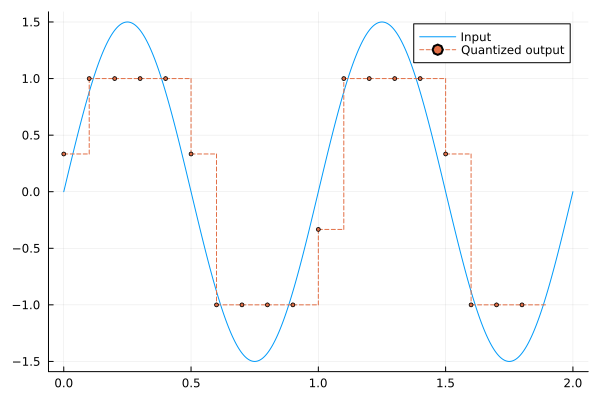

Different quantization modes

With the default option midrise = true, the output of the quantizer is always between y_min and y_max inclusive, and the number of distinct levels it can take is 2^bits. The possible values are given by:

bits = 2; y_min = -1; y_max = 1
collect(range(y_min, stop=y_max, length=2^bits))
# 4-element Vector: [-1.0, -0.333, 0.333, 1.0]

Notably, these possible levels do not include 0. If midrise = false, a mid-tread quantizer is used instead.

The mid-rise quantizer has a rise at the middle of the interval, while the mid-tread mode has a flat region (a tread) centered around the middle of the interval.

The default option midrise = true includes both end points as possible output values, while midrise = false does not include the upper limit.

Sampling with AD effects

The SampleWithADEffects component combines an ideal Sampler, a NormalNoise, and a Quantization component to simulate the undesirable but practically occurring effects of sampling, noise, and quantization in an AD converter. The component has the connectors u and y, where the input is the continuous-time signal to be sampled, and the output is the quantized, noisy discrete-time signal. Example:

"""
Demonstrates the SampleWithADEffects component which combines
sampling, noise, and quantization in a single block.
"""
test component PracticalSamplerDemo
  input_signal = BlockComponents.Sources.Sine(amplitude = 1.2, frequency = 1) {^input_signal}
  sampling = DiscreteComponents.SampleWithADEffects(bits = 3, y_min = -1, y_max = 1, sigma = 0.1, quantized = true) {^sampling}
  terminator = BlockComponents.Routing.Terminator() {^terminator}
  periodicclock = DiscreteComponents.PeriodicClock(dt = 0.1) {^periodicclock}
relations
  connect(input_signal.y, sampling.u) {^id5}
  connect(sampling.y, terminator.u, periodicclock.y) {^id6}
metadata {
  "_links": {
    "input_signal": {
      "Dyad": {
        "placement": {
          "diagram": {"iconName": "default", "x1": 20, "y1": 20, "x2": 220, "y2": 220, "rot": 0}
        },
        "tags": []
      }
    },
    "sampling": {
      "Dyad": {
        "placement": {
          "diagram": {"iconName": "default", "x1": 280, "y1": 20, "x2": 480, "y2": 220, "rot": 0}
        },
        "tags": []
      }
    },
    "terminator": {
      "Dyad": {
        "placement": {
          "diagram": {"iconName": "default", "x1": 710, "y1": 70, "x2": 810, "y2": 170, "rot": 0}
        },
        "tags": []
      }
    },
    "periodicclock": {
      "Dyad": {
        "placement": {
          "diagram": {"iconName": "default", "x1": 430, "y1": 330, "x2": 330, "y2": 430, "rot": 0}
        },
        "tags": []
      }
    },
    "id5": {"Dyad": {"edges": [{"S": 1, "M": [], "E": 2}], "renderStyle": "standard"}},
    "id6": {
      "Dyad": {
        "edges": [
          {"S": 1, "M": [], "E": -1},
          {"S": -1, "M": [], "E": 2},
          {"S": 3, "M": [{"x": 600, "y": 380}], "E": -1}
        ],
        "junctions": [{"x": 600, "y": 120}],
        "renderStyle": "standard"
      }
    }
  }
}
end

analysis PracticalSamplerDemoAnalysis
  extends TransientAnalysis(stop = 2.0)
  model = PracticalSamplerDemo()
end

result = PracticalSamplerDemoAnalysis()
model = artifacts(result, :SimplifiedSystem)
plot(result; idxs = [model.input_signal.y, model.sampling.y],
    labels = ["Input" "AD converted output"])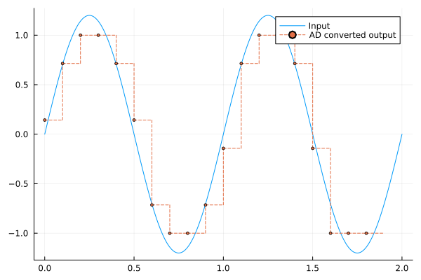

Quantization is optional and turned off by default. In the example above, we turn it on with quantized = true. The noise is Gaussian white noise with standard deviation sigma, and the quantization is a 3-bit midrise quantizer (8 output levels) with limits y_min and y_max. Limits have to be provided when quantization is used.

Things to notice in the plot:

• The sampled signal is saturated at the quantization limits +-1.

• The noise is added to the signal before quantization, which means that the sampled signal has distinct output levels only.

• 0 is not a possible output value. In situations where 0 is an important value (such as in the presence of integration of a quantized value that is expected to be close to 0), the mid-tread quantizer should be used instead by passing midrise = false.