
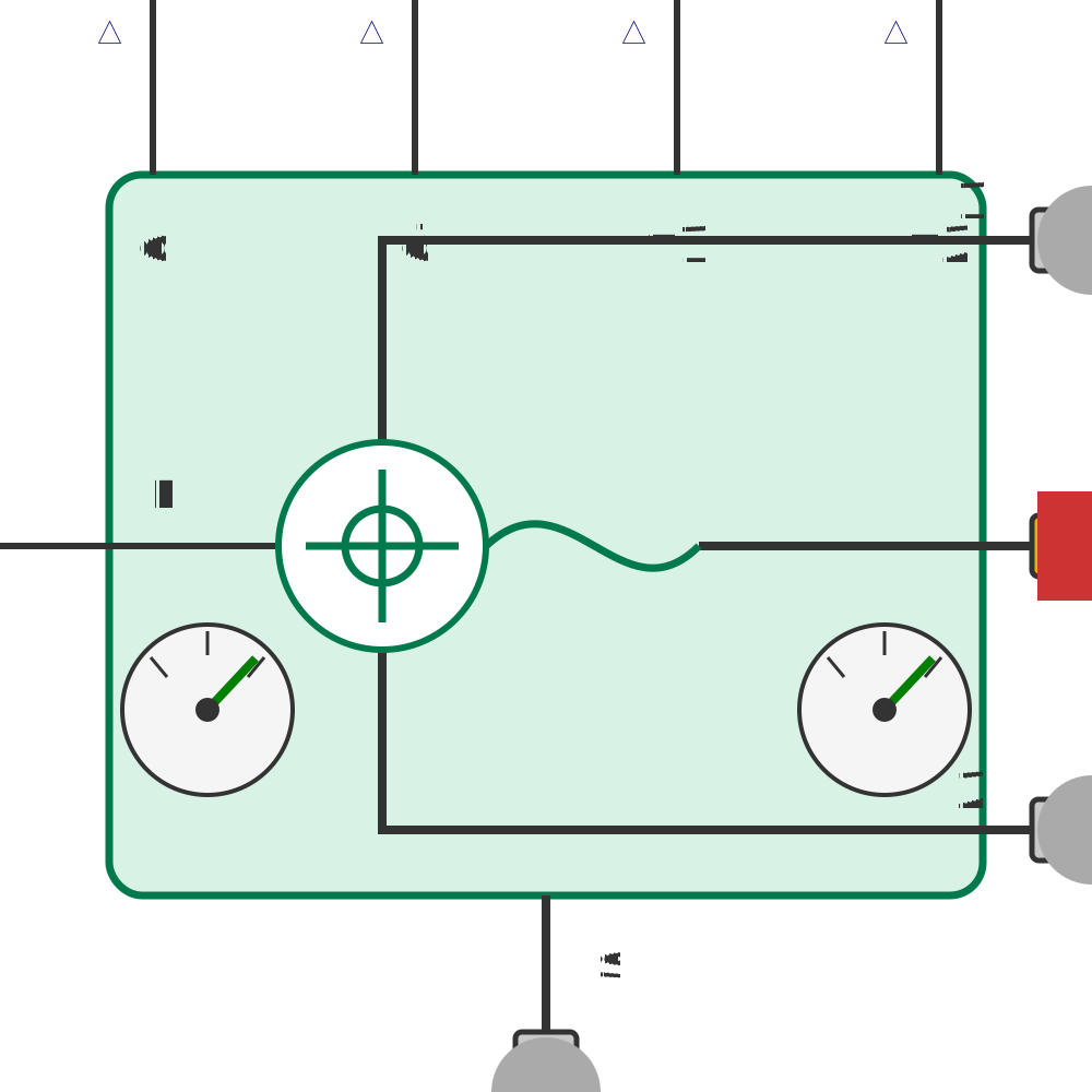
PlanarMechanics.examples.two_joint_robot.InverseKinematicsDriver
Drives an inverse robot model in Cartesian tool space: the tool-flange position of the inverse model (connected at frame) is constrained to follow the reference position r_ref without applying any force there, while the joints (connected at flange1, flange2) are actuated by unknown torques. The unknown torques are determined by the position constraint and therefore solve the inverse kinematics and inverse dynamics of the reference motion simultaneously: tau1, tau2 constitute a computed-torque feedforward signal, and the joint angles q and velocities qd measured on the inverse model constitute joint-space references for feedback controllers.
The position constraint is differentiated twice by index reduction, so the reference signal must be smooth (e.g. generated by KinematicPTPBoundedJerk).
Usage
MultibodyComponents.PlanarMechanics.examples.two_joint_robot.InverseKinematicsDriver()
Connectors
r_ref- This connector represents a real signal as an input to a component (RealInput)frame- Coordinate system (2-dim.) fixed to the component with one cut-force and cut-torque.
All variables are resolved in the planar world frame. (Frame2D)
flange1- This connector represents a rotational spline with angle and torque as the potential and flow variables, respectively. (Spline)flange2- This connector represents a rotational spline with angle and torque as the potential and flow variables, respectively. (Spline)support- This connector represents a rotational spline with angle and torque as the potential and flow variables, respectively. (Spline)q- This connector represents a real signal as an output from a component (RealOutput)qd- This connector represents a real signal as an output from a component (RealOutput)tau1- This connector represents a real signal as an output from a component (RealOutput)tau2- This connector represents a real signal as an output from a component (RealOutput)
Behavior
Source
"""
Drives an inverse robot model in Cartesian tool space: the tool-flange position of
the inverse model (connected at `frame`) is constrained to follow the reference
position `r_ref` without applying any force there, while the joints (connected at
`flange1`, `flange2`) are actuated by unknown torques. The unknown torques are
determined by the position constraint and therefore solve the inverse kinematics
and inverse dynamics of the reference motion simultaneously: `tau1`, `tau2`
constitute a computed-torque feedforward signal, and the joint angles `q` and
velocities `qd` measured on the inverse model constitute joint-space references
for feedback controllers.

The position constraint is differentiated twice by index reduction, so the
reference signal must be smooth (e.g. generated by `KinematicPTPBoundedJerk`).
"""
component InverseKinematicsDriver
  "Cartesian reference position of the tool flange"
  r_ref = [RealInput() for i in 1:2] {
    "Dyad": {
      "placement": {
        "diagram": {"iconName": "default", "x1": -40, "y1": 460, "x2": 60, "y2": 560, "rot": 0}
      },
      "tags": []
    }
  }
  "Frame driving the tool flange of the inverse model"
  frame = Frame2D() {
    "Dyad": {
      "placement": {
        "diagram": {"iconName": "default", "x1": 950, "y1": 450, "x2": 1050, "y2": 550, "rot": 0}
      },
      "tags": []
    }
  }
  "Flange driving joint 1 of the inverse model"
  flange1 = Spline() {
    "Dyad": {
      "placement": {
        "diagram": {"iconName": "default", "x1": 950, "y1": 170, "x2": 1050, "y2": 270, "rot": 0}
      },
      "tags": []
    }
  }
  "Flange driving joint 2 of the inverse model"
  flange2 = Spline() {
    "Dyad": {
      "placement": {
        "diagram": {"iconName": "default", "x1": 950, "y1": 710, "x2": 1050, "y2": 810, "rot": 0}
      },
      "tags": []
    }
  }
  "Support flange of the torque sources"
  support = Spline() {
    "Dyad": {
      "placement": {
        "diagram": {"iconName": "default", "x1": 450, "y1": 950, "x2": 550, "y2": 1050, "rot": 0}
      },
      "tags": []
    }
  }
  "Joint angles of the inverse model realizing the reference motion"
  q = [RealOutput() for i in 1:2] {
    "Dyad": {
      "placement": {
        "diagram": {"iconName": "default", "x1": 90, "y1": -60, "x2": 190, "y2": 40, "rot": 270}
      },
      "tags": []
    }
  }
  "Joint velocities of the inverse model realizing the reference motion"
  qd = [RealOutput() for i in 1:2] {
    "Dyad": {
      "placement": {
        "diagram": {"iconName": "default", "x1": 330, "y1": -60, "x2": 430, "y2": 40, "rot": 270}
      },
      "tags": []
    }
  }
  "Torque required to realize the reference motion of joint 1"
  tau1 = RealOutput() {
    "Dyad": {
      "placement": {
        "diagram": {"iconName": "default", "x1": 570, "y1": -60, "x2": 670, "y2": 40, "rot": 270}
      },
      "tags": []
    }
  }
  "Torque required to realize the reference motion of joint 2"
  tau2 = RealOutput() {
    "Dyad": {
      "placement": {
        "diagram": {"iconName": "default", "x1": 810, "y1": -60, "x2": 910, "y2": 40, "rot": 270}
      },
      "tags": []
    }
  }
  pos = MultibodyComponents.PlanarMechanics.PrescribedPosition(fixed_orientation = false, apply_force = false) {}
  utau1 = UnknownTorqueSource() {}
  utau2 = UnknownTorqueSource() {}
  ang1 = RotationalComponents.Sensors.AngleSensor() {
    "Dyad": {
      "placement": {
        "diagram": {"iconName": "default", "x1": 250, "y1": 570, "x2": 150, "y2": 670, "rot": 0}
      },
      "tags": []
    }
  }
  ang2 = RotationalComponents.Sensors.AngleSensor() {
    "Dyad": {
      "placement": {
        "diagram": {"iconName": "default", "x1": 250, "y1": 720, "x2": 150, "y2": 820, "rot": 0}
      },
      "tags": []
    }
  }
  vel1 = RotationalComponents.Sensors.VelocitySensor() {
    "Dyad": {
      "placement": {
        "diagram": {"iconName": "default", "x1": 290, "y1": 600, "x2": 390, "y2": 700, "rot": 0}
      },
      "tags": []
    }
  }
  vel2 = RotationalComponents.Sensors.VelocitySensor() {
    "Dyad": {
      "placement": {
        "diagram": {"iconName": "default", "x1": 650, "y1": 630, "x2": 750, "y2": 730, "rot": 270}
      },
      "tags": []
    }
  }
relations
  connect(r_ref[1], pos.r_x)
  connect(r_ref[2], pos.r_y)
  connect(pos.frame_b, frame)
  connect(utau1.spline, ang1.spline, vel1.spline, flange1) {
    "Dyad": {
      "edges": [
        {"S": 1, "M": [{"x": 500, "y": 500}, {"x": 500, "y": 620}], "E": 2},
        {"S": 2, "M": [{"x": 250, "y": 650}], "E": 3},
        {"S": 3, "M": [{"x": 260, "y": 650}, {"x": 260, "y": 220}], "E": 4}
      ],
      "renderStyle": "standard"
    }
  }
  connect(utau2.spline, ang2.spline, vel2.spline, flange2) {
    "Dyad": {
      "edges": [
        {"S": 1, "M": [{"x": 500, "y": 500}, {"x": 500, "y": 770}], "E": 2},
        {"S": 2, "M": [{"x": 250, "y": 730}], "E": 3},
        {"S": 3, "M": [{"x": 700, "y": 760}], "E": 4}
      ],
      "renderStyle": "standard"
    }
  }
  connect(utau1.support, support)
  connect(utau2.support, support)
  connect(ang1.phi, q[1]) {
    "Dyad": {
      "edges": [{"S": 1, "M": [{"x": 140, "y": 620}], "E": 2}],
      "renderStyle": "standard"
    }
  }
  connect(ang2.phi, q[2]) {
    "Dyad": {
      "edges": [{"S": 1, "M": [{"x": 140, "y": 770}], "E": 2}],
      "renderStyle": "standard"
    }
  }
  connect(vel1.w, qd[1]) {
    "Dyad": {
      "edges": [{"S": 1, "M": [{"x": 390, "y": 245}, {"x": 380, "y": 245}], "E": 2}],
      "renderStyle": "standard"
    }
  }
  connect(vel2.w, qd[2]) {
    "Dyad": {
      "edges": [{"S": 1, "M": [{"x": 530, "y": 245}, {"x": 380, "y": 245}], "E": 2}],
      "renderStyle": "standard"
    }
  }
  connect(utau1.tau, tau1)
  connect(utau2.tau, tau2)
metadata {
  "Dyad": {"icons": {"default": "dyad://MultibodyComponents/InverseKinematicsDriver.svg"}}
}
end
Flattened Source
"""
Drives an inverse robot model in Cartesian tool space: the tool-flange position of
the inverse model (connected at `frame`) is constrained to follow the reference
position `r_ref` without applying any force there, while the joints (connected at
`flange1`, `flange2`) are actuated by unknown torques. The unknown torques are
determined by the position constraint and therefore solve the inverse kinematics
and inverse dynamics of the reference motion simultaneously: `tau1`, `tau2`
constitute a computed-torque feedforward signal, and the joint angles `q` and
velocities `qd` measured on the inverse model constitute joint-space references
for feedback controllers.

The position constraint is differentiated twice by index reduction, so the
reference signal must be smooth (e.g. generated by `KinematicPTPBoundedJerk`).
"""
component InverseKinematicsDriver
  "Cartesian reference position of the tool flange"
  r_ref = [RealInput() for i in 1:2] {
    "Dyad": {
      "placement": {
        "diagram": {"iconName": "default", "x1": -40, "y1": 460, "x2": 60, "y2": 560, "rot": 0}
      },
      "tags": []
    }
  }
  "Frame driving the tool flange of the inverse model"
  frame = Frame2D() {
    "Dyad": {
      "placement": {
        "diagram": {"iconName": "default", "x1": 950, "y1": 450, "x2": 1050, "y2": 550, "rot": 0}
      },
      "tags": []
    }
  }
  "Flange driving joint 1 of the inverse model"
  flange1 = Spline() {
    "Dyad": {
      "placement": {
        "diagram": {"iconName": "default", "x1": 950, "y1": 170, "x2": 1050, "y2": 270, "rot": 0}
      },
      "tags": []
    }
  }
  "Flange driving joint 2 of the inverse model"
  flange2 = Spline() {
    "Dyad": {
      "placement": {
        "diagram": {"iconName": "default", "x1": 950, "y1": 710, "x2": 1050, "y2": 810, "rot": 0}
      },
      "tags": []
    }
  }
  "Support flange of the torque sources"
  support = Spline() {
    "Dyad": {
      "placement": {
        "diagram": {"iconName": "default", "x1": 450, "y1": 950, "x2": 550, "y2": 1050, "rot": 0}
      },
      "tags": []
    }
  }
  "Joint angles of the inverse model realizing the reference motion"
  q = [RealOutput() for i in 1:2] {
    "Dyad": {
      "placement": {
        "diagram": {"iconName": "default", "x1": 90, "y1": -60, "x2": 190, "y2": 40, "rot": 270}
      },
      "tags": []
    }
  }
  "Joint velocities of the inverse model realizing the reference motion"
  qd = [RealOutput() for i in 1:2] {
    "Dyad": {
      "placement": {
        "diagram": {"iconName": "default", "x1": 330, "y1": -60, "x2": 430, "y2": 40, "rot": 270}
      },
      "tags": []
    }
  }
  "Torque required to realize the reference motion of joint 1"
  tau1 = RealOutput() {
    "Dyad": {
      "placement": {
        "diagram": {"iconName": "default", "x1": 570, "y1": -60, "x2": 670, "y2": 40, "rot": 270}
      },
      "tags": []
    }
  }
  "Torque required to realize the reference motion of joint 2"
  tau2 = RealOutput() {
    "Dyad": {
      "placement": {
        "diagram": {"iconName": "default", "x1": 810, "y1": -60, "x2": 910, "y2": 40, "rot": 270}
      },
      "tags": []
    }
  }
  pos = MultibodyComponents.PlanarMechanics.PrescribedPosition(fixed_orientation = false, apply_force = false) {}
  utau1 = UnknownTorqueSource() {}
  utau2 = UnknownTorqueSource() {}
  ang1 = RotationalComponents.Sensors.AngleSensor() {
    "Dyad": {
      "placement": {
        "diagram": {"iconName": "default", "x1": 250, "y1": 570, "x2": 150, "y2": 670, "rot": 0}
      },
      "tags": []
    }
  }
  ang2 = RotationalComponents.Sensors.AngleSensor() {
    "Dyad": {
      "placement": {
        "diagram": {"iconName": "default", "x1": 250, "y1": 720, "x2": 150, "y2": 820, "rot": 0}
      },
      "tags": []
    }
  }
  vel1 = RotationalComponents.Sensors.VelocitySensor() {
    "Dyad": {
      "placement": {
        "diagram": {"iconName": "default", "x1": 290, "y1": 600, "x2": 390, "y2": 700, "rot": 0}
      },
      "tags": []
    }
  }
  vel2 = RotationalComponents.Sensors.VelocitySensor() {
    "Dyad": {
      "placement": {
        "diagram": {"iconName": "default", "x1": 650, "y1": 630, "x2": 750, "y2": 730, "rot": 270}
      },
      "tags": []
    }
  }
relations
  connect(r_ref[1], pos.r_x)
  connect(r_ref[2], pos.r_y)
  connect(pos.frame_b, frame)
  connect(utau1.spline, ang1.spline, vel1.spline, flange1) {
    "Dyad": {
      "edges": [
        {"S": 1, "M": [{"x": 500, "y": 500}, {"x": 500, "y": 620}], "E": 2},
        {"S": 2, "M": [{"x": 250, "y": 650}], "E": 3},
        {"S": 3, "M": [{"x": 260, "y": 650}, {"x": 260, "y": 220}], "E": 4}
      ],
      "renderStyle": "standard"
    }
  }
  connect(utau2.spline, ang2.spline, vel2.spline, flange2) {
    "Dyad": {
      "edges": [
        {"S": 1, "M": [{"x": 500, "y": 500}, {"x": 500, "y": 770}], "E": 2},
        {"S": 2, "M": [{"x": 250, "y": 730}], "E": 3},
        {"S": 3, "M": [{"x": 700, "y": 760}], "E": 4}
      ],
      "renderStyle": "standard"
    }
  }
  connect(utau1.support, support)
  connect(utau2.support, support)
  connect(ang1.phi, q[1]) {
    "Dyad": {
      "edges": [{"S": 1, "M": [{"x": 140, "y": 620}], "E": 2}],
      "renderStyle": "standard"
    }
  }
  connect(ang2.phi, q[2]) {
    "Dyad": {
      "edges": [{"S": 1, "M": [{"x": 140, "y": 770}], "E": 2}],
      "renderStyle": "standard"
    }
  }
  connect(vel1.w, qd[1]) {
    "Dyad": {
      "edges": [{"S": 1, "M": [{"x": 390, "y": 245}, {"x": 380, "y": 245}], "E": 2}],
      "renderStyle": "standard"
    }
  }
  connect(vel2.w, qd[2]) {
    "Dyad": {
      "edges": [{"S": 1, "M": [{"x": 530, "y": 245}, {"x": 380, "y": 245}], "E": 2}],
      "renderStyle": "standard"
    }
  }
  connect(utau1.tau, tau1)
  connect(utau2.tau, tau2)
metadata {
  "Dyad": {"icons": {"default": "dyad://MultibodyComponents/InverseKinematicsDriver.svg"}}
}
end
Test Cases
No test cases defined.
Related
Examples
Experiments
Analyses