
Array Variables in Clocked Components
Clocked variables and connectors may be arrays, which is what makes shift registers, MIMO discrete-time systems and vector-valued discrete logic expressible. This page collects the patterns and the rough edges.
See Discrete-Time Modeling for clocks and shift operators, Arrays for array syntax in general, and Clocks for the clock-annotation grammar.
Array-valued clocked variables
An array variable is declared as usual, and each element may carry its own clocked equation. The dimension must be a literal or a structural parameter.
The canonical use is a shift register: element 1 takes the current input and every other element takes the previous value of its neighbour. Averaging the register gives a moving-average filter: Download as a Dyad projectdiscretearrays.zipOpen in Dyad Studio
"""
Moving average over the last `N` samples, implemented as an array-valued shift
register, with a whole-array initial condition at shift -1.
"""
component WindowAverage@[input clk extends Discrete]
  "Input signal"
  u = Dyad.RealInput@[clk]()
  "Averaged output"
  y = Dyad.RealOutput@[clk]()
  "Number of samples to average over"
  structural parameter N::Integer = 4
  "The shift register"
  variable taps::Real[N]
relations
  taps[1]@clk = u@clk
  for i in 2:N
    taps[i]@clk = taps[i - 1]@(clk-1)
  end
  initial taps@(clk-1) = fill(0.0, N)
  y = sum(taps) / N
end
Two things to note. The for loop is unrolled at compile time, because N is a structural parameter — this is N-1 equations, not a runtime loop. And sum works directly on the symbolic array.
The initial condition is not optional, and it must cover the array as a whole. Omitting it fails with
An initial value must be specified for shifted variable taps(t) at shift -1and the element-by-element form, for i in 1:N initial taps[i]@(clk-1) = 0.0 end, fails differently — KeyError: key (taps(t))[1] not found — because the synchronous compiler does not match scalarized initial conditions back to the array they belong to. Write initial taps@(clk-1) = fill(0.0, N).
The library's MovingAverageFilter is this component, with an initialization parameter instead of a hard-coded zero — see Initializing Discrete-Time Components. Reach for it rather than writing your own; WindowAverage is here to show the array mechanics.
Wiring it to a sampled noisy sine shows the smoothing:
"""
`WindowAverage` smoothing a noisy sampled sine.
"""
test component WindowAverageDemo
  source = BlockComponents.Sources.Sine(amplitude = 1.0, frequency = 1.0)
  sampling = DiscreteComponents.SampleWithADEffects(sigma = 0.15, quantized = false)
  clock = DiscreteComponents.PeriodicClock(dt = 0.02)
  avg = WindowAverage(N = 8)
relations
  connect(source.y, sampling.u)
  connect(sampling.y, clock.y, avg.u)
end

analysis WindowAverageDemoAnalysis
  extends TransientAnalysis(stop = 2.0)
  model = WindowAverageDemo()
endusing Plots
using DyadInterface
result = WindowAverageDemoAnalysis()
model = artifacts(result, :SimplifiedSystem)
p1 = plot(result; idxs = model.sampling.y, title = "Noisy samples")
p2 = plot(result; idxs = model.avg.y, title = "8-sample average")
plot(p1, p2; layout = (2, 1), legend = false, xlabel = "t", ylabel = "Signal",
size = (600, 420),
plot_title = "Array shift register as a moving-average filter")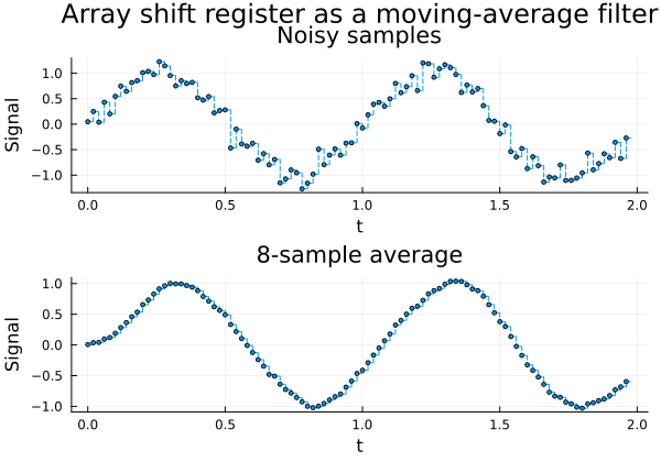
Whole-array equations
An equation may also be written for an entire array at once, with matrix–vector products on the right-hand side. This is how DiscreteStateSpace expresses a linear system:
  x@clk = A * x@(clk-1) + B * (u@clk - u0)
  y@clk = C * x@(clk-1) + D * (u@clk - u0) + y0
Remember the negative-shift convention: x@(clk-1) is the current state and x@clk is the one being computed, so these two lines are
Array connectors
A component can expose a vector of connectors by building them with a comprehension. DiscreteStateSpace does this for its inputs and outputs:
component DiscreteStateSpace@[input clk extends Discrete]
  u = [RealInput@[clk]() for i in 1:nu] {^u}
  y = [RealOutput@[clk]() for i in 1:ny] {^y}
  structural parameter nx::Integer = 2
  structural parameter nu::Integer = 1
  structural parameter ny::Integer = 1
  parameter A::Real[nx, nx] = fill(0.0, nx, nx)
  parameter B::Real[nx, nu] = fill(1.0, nx, nu)
  parameter C::Real[ny, nx] = fill(1.0, ny, nx)
  parameter D::Real[ny, nu] = fill(0.0, ny, nu)
  variable x::Real[nx]
  ...
end
Individual elements are then connected as connect(src.y, ss.u[1]).
Writing matrix literals
Dyad array literals are comma-separated, and a matrix is a list of rows — there is no MATLAB-style ; row separator or space-separated column syntax. A
parameter A::Real[2, 2] = [[0.9, 0.05], [0.0, 0.85]]
parameter B::Real[2, 1] = [[0.0], [0.1]]
parameter C::Real[1, 2] = [[1.0, 0.0]]
Writing [0.9 0.05; 0.0 0.85] instead is a parse error. fill is available for uniform matrices, which is how DiscreteStateSpace spells its own defaults (fill(0.0, nx, nx)).
Array initial conditions
Vector-valued state uses the array variants of the initialization enum, InitialStateArray(x0) and InitialOutputArray(y0) — see Initializing Discrete-Time Components for the scalar counterparts. Components with array state generally reject the scalar variants, and vice versa, because the shapes cannot be reconciled.
Discrete state-space blocks
DiscreteStateSpace combines everything above — array connectors, array state, whole-array equations and array initial conditions — into a MIMO linear block:
ss = DiscreteComponents.DiscreteStateSpace(
    nx = 2, nu = 1, ny = 1,
    A = [[0.9, 0.05], [0.0, 0.85]],
    B = [[0.0], [0.1]],
    C = [[1.0, 0.0]],
    D = [[0.0]],
    initialization = DiscreteComponents.InitialCondition.InitialStateArray(x0 = [0.5, 0.0]))
Reading array results
Indexing a solution with a vector-valued clocked variable returns a vector of vectors, one entry per sample. Flatten it into a matrix when you want to work with it numerically:
sol = artifacts(result, :RawSolution)
X = reduce(hcat, sol[model.avg.taps])   # N × number-of-samples
Individual elements can be indexed directly, e.g. model.avg.taps[1]. See Reading results for the clocked-variable time grid.
Limitations
A clock cannot be attached to an array connection. A clock output is scalar, so a
PeriodicClockmust be connected to a scalar signal in the partition — as in the example above, where the clock joins the sampler output rather than an array port.A clocked array read at a negative shift needs an initial condition, given for the whole array. There is no implicit zero, and the element-wise form does not register — write
initial taps@(clk-1) = fill(0.0, N).Use floating-point literals in array element equations. Writing
0rather than0.0in an equation for one element of aRealarray can leave the array with mixed element types, which fails when the model is lowered for code generation. Write0.0.
See also
Discrete-Time Modeling — clocks, partitions and reading results
Sampled-Data Systems — combining discrete-time and continuous-time models
Initializing Discrete-Time Components — the initialization enum, including the array variants
DiscreteStateSpaceandMovingAverageFilter— the components shown hereControlSystems.jl — building the
A,B,C,Dmatrices for a discrete-time design