Getting Started with Dyad Studio
In this section, we will discuss the basics for using Dyad for modeling and simulation. This includes:
How to use the Dyad VS Code extension
How to create a Dyad model
How to compile a model for simulation
How to run basic simulations
How to bring in standard libraries and compose models from components
Before starting this tutorial, install Dyad Studio.
First Step: Creating a Component Library
In Dyad, all new components must be created in a component library. Thus our first step will be to create a new component library which we can use as a playground.
In Dyad Studio, you can create a new library by opening the Command Palette in VS Code (⇧ ⌘ P on MacOS, Ctrl-Shift-P on Windows). From the Command Palette, type Dyad and you should see the following options:
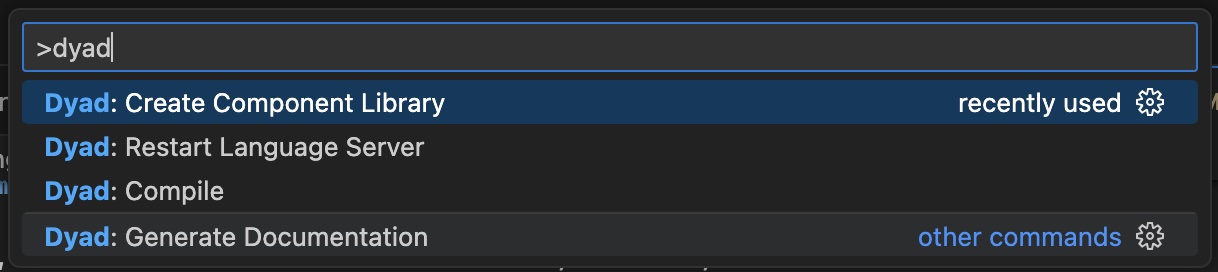
Select Dyad: Create Component Library from the list. You will then be prompted for the name of the library with a dialog like this one (although the appearance of the VS Code UI elements can differ from operating system to operating system).

It is suggested that the library name end in Components as a simple way of indicating that the package is a Dyad component library. But it isn't strictly necessary that it end with Components. But it does need to be both a valid Julia identifier and a valid directory name. As such, the names are currently limited to include only letters to ensure both constraints are satisified.
Once you enter a name, you'll be prompted for a directory to store the new package in. The Create Component Library command will create a new directory inside the directory you select. Furthermore, the new directory will have the same name as the package. Said another way, whatever directory you select will get another directory created inside of it.
When the library creation process is done, a new Visual Studio Code window will open in the newly created directory.
NOTE
If you want to create a new Dyad component library with the Dyad CLI, you can simply run:
$ dyad create <LibraryName>...from any directory and this command will create a new directory called with the library name you provided.
Setting Up Your Environment
The generated library includes a sample component and analysis. Open the library in Dyad Studio and wait for initialization to finish. Studio installs the library's Julia dependencies automatically with its default settings.
The first setup and analysis run can take several minutes while packages download and precompile. Subsequent runs are faster; see the FAQ for more about precompilation.
Running Our First Simulation: Lumped Thermal Model
Before getting to anything fancy, let's see how to use Dyad to define a lumped thermal model and simulate to see the solution. We use Newton's Law of cooling/heating which can be represented by the following simple linear ODE:
In the rest of this section, we will:
Look at a component representing this lumped thermal system.
Discuss an analysis for simulating the thermal response of the system.
Explore the analysis results via plots and other solution artifacts.
Newton's Law of Cooling/Heating
TIP
By whatever means you created the library, for the rest of this section we will assume you have opened the Dyad library in Visual Studio Code.
As mentioned previously, the result of all of this will be a new Julia package pre-configured for use as a Dyad library. Included will be a Project.toml file that identifies the directory as a Julia package and lists its (initial) dependencies. You will also find a dyad directory that includes a file called hello.dyad. In there you will find two things. First, you'll find a Dyad component definition that should look something like this:
# A simple lumped thermal model
component Hello
  # Ambient temperature
  parameter T_inf::Temperature = 300
  # Initial temperature
  parameter T0::Temperature = 320
  # Convective heat transfer coefficient
  parameter h::CoefficientOfHeatTransfer = 0.7
  # Surface area
  parameter A::Area = 1.0
  # Mass of thermal capacitance
  parameter m::Mass = 0.1
  # Specific Heat
  parameter c_p::SpecificHeatCapacity = 1.2
  variable T::Temperature
relations
  # Specify initial conditions
  initial T = T0
  # Newton's law of cooling/heating
  m*c_p*der(T) = h*A*(T_inf-T)
end
In addition you should also find an analysis that looks something like this:
analysis World
  extends TransientAnalysis(stop=10)
  model = Hello(T_inf=T_inf, h=h)
  parameter T_inf::Temperature = 300
  parameter h::CoefficientOfHeatTransfer = 0.7
end
The Hello definition describes a first order system. The temperature response of the system is contained in the variable T. The various physical properties of the material are represented by the mass (m), the surface area (A), and the specific heat capacity (c_p). The environmental conditions are represented by the ambient temperature (T_inf) and the convective heat transfer coefficient (h). Finally, the initial temperature for T at the start of the simulation is prescribed using the parameter T0 (and the initial T = T0 relation).
Simulating the Thermal Model
Save hello.dyad. In the Analyses sidebar, click Run Analysis (the play button) beside World.
Dyad Studio compiles the model and runs the transient simulation of Hello with T_inf=300 and h=0.7. It displays the simulation plot and leaves the result in the Julia REPL as solution.
The plot shows T cooling from solution in the Julia REPL for further plots and artifact queries. To plot the response again with Plots.jl, enter:
using Plots
plot(solution)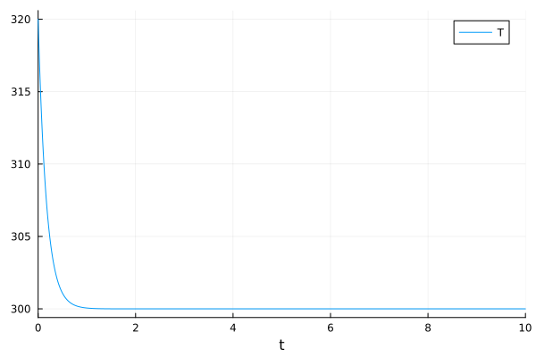
Interactively Modifying Analyses
The World analysis exposes the ambient temperature and heat transfer coefficient as parameters and passes them to Hello. To simulate heating, change their values in hello.dyad:
analysis World
  extends TransientAnalysis(stop=10)
  model = Hello(T_inf=T_inf, h=h)
  parameter T_inf::Temperature = 400
  parameter h::CoefficientOfHeatTransfer = 0.2
end
Save the file and click Run Analysis beside World again. The new result replaces solution in the Julia REPL. Plot it with the same command:
plot(solution)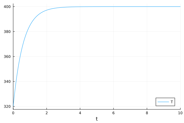
The body now heats toward the ambient temperature of
Obtaining Artifacts from an Analysis
An analysis exposes plots, tables, and other results as artifacts. List the artifacts available from the latest run:
using DyadInterface
artifacts(solution)
6-element Vector{Symbol}:
:SimulationSolutionPlot
:SimulationSolutionTable
:ObservablesTable
:RawSolution
:SimplifiedSystem
:InitialSystemThe transient result includes a plot and a solution table. Retrieve the table with:
table = artifacts(solution, :SimulationSolutionTable)| Row | timestamp | T(t) |
|---|---|---|
| Float64 | Float64 | |
| 1 | 0.0 | 320.0 |
| 2 | 0.0270361 | 323.525 |
| 3 | 0.0800624 | 329.993 |
| 4 | 0.145411 | 337.218 |
| 5 | 0.22629 | 345.135 |
| 6 | 0.320872 | 353.136 |
| 7 | 0.430032 | 360.932 |
| 8 | 0.552807 | 368.161 |
| 9 | 0.689319 | 374.64 |
| 10 | 0.839177 | 380.245 |
| 11 | 1.00251 | 384.953 |
| 12 | 1.17944 | 388.796 |
| 13 | 1.37044 | 391.85 |
| 14 | 1.57615 | 394.216 |
| 15 | 1.79754 | 396.001 |
| 16 | 2.0359 | 397.312 |
| 17 | 2.29288 | 398.248 |
| 18 | 2.57057 | 398.897 |
| 19 | 2.87162 | 399.332 |
| 20 | 3.19933 | 399.613 |
| 21 | 3.55786 | 399.787 |
| 22 | 3.95252 | 399.89 |
| 23 | 4.39011 | 399.947 |
| 24 | 4.87949 | 399.976 |
| 25 | 5.4325 | 399.991 |
| 26 | 6.06518 | 399.997 |
| 27 | 6.80004 | 399.999 |
| 28 | 7.66961 | 400.0 |
| 29 | 8.72283 | 400.0 |
| 30 | 10.0 | 400.0 |
As described in the TransientAnalysis documentation, this returns a data table of the solution values that can be used to serialize the information.
Each analysis provides its own artifacts. A controls analysis can provide Bode plots, while a surrogate analysis can provide a trained neural network. The analysis documentation describes its available results.
Using Model Libraries and Composing Components: Generating an RLC Circuit
Dyad supports acausal modeling which means it has the ability to take pre-built model components and stich them together to quickly build complex models. Let's show this off by building a simple RLC circuit. The components for an RLC circuit are defined in the ElectricalComponents standard library, so let's first pull that library in:
using Pkg
Pkg.add("ElectricalComponents")
This is just one of many standard libraries included in Dyad, peruse the documentation pages on the component libraries to see all of the prebuilt models for fluids, hydraulics, mechanical systems, and much more!
Create dyad/rlc.dyad in your library. Start with a partial component that defines the shared two-pin interface and current balance. Its metadata places the built-in positive and negative pin icons on opposite edges:
partial component TwoPin
  p = Pin() {^p}
  n = Pin() {^n}
  variable v::Voltage
  variable i::Current
relations
  v = p.v - n.v
  i = p.i
  p.i + n.i = 0
metadata {
  "_links": {
    "p": {
      "Dyad": {
        "placement": {"icon": {"iconName": "pos", "x1": -50, "y1": 450, "x2": 50, "y2": 550}}
      }
    },
    "n": {
      "Dyad": {
        "placement": {"icon": {"iconName": "neg", "x1": 950, "y1": 450, "x2": 1050, "y2": 550}}
      }
    }
  }
}
end
The partial component leaves the voltage–current relationship open. Derive StepVoltage from it and add the source's voltage law:
Assemble the local voltage source with ElectricalComponents' resistor, inductor, capacitor, and ground:
Notice this is the same syntax as how we defined the Hello component, but now instead of defining all of the relational equations from scratch, we are pulling in these equations from pre-defined components and using the connect relation to compose them together. And just like before, we can use a TransientAnalysis to simulate this model. Let's build a simulation of this component and inspect its results. Add this analysis to dyad/rlc.dyad:
analysis SimRLC
  extends TransientAnalysis(stop=10, abstol=1m, reltol=1m)
  model = RLC()
end
Save rlc.dyad and click Run Analysis beside SimRLC in the Analyses sidebar. The circuit's simulation result is now solution in the Julia REPL. Plot it there:
using DyadInterface, Plots
plot(solution)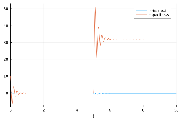
By default it only plots what was solved, but the RLC has many more aspects to its model. We can use the idxs command in the plot to show other solved values:
sys = artifacts(solution, :SimplifiedSystem)
plot(solution; idxs = [sys.capacitor.v, sys.resistor.i])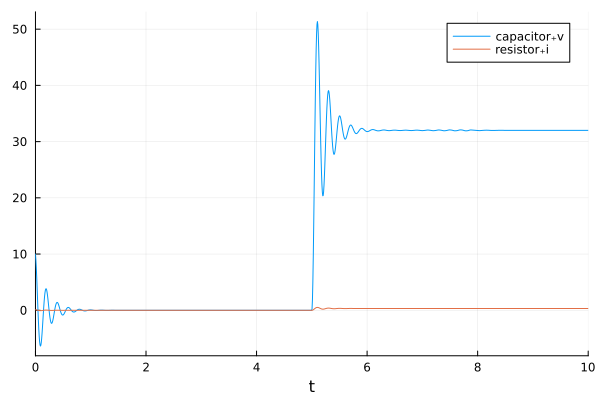
Next Steps and Where to Learn More
Congrats! You now know how to build some basic components in Dyad, run simulations, and stitch together pre-built components for more complex models. But there are lots of other features to explore and much more to learn. Some recommended next steps are:
See how to construct more complex models using the standard libraries. This is recommended if you want to get up and running with complex simulations quickly.
Learn more about how acausal modeling works by building the RLC circuit from scratch. This is for if you care about the details: how was everything defined? How does it know equations to simulate? Etc.
Want more details on the Dyad language? Check out the Dyad Language Guide
Learn how to do more with your models by seeing analysis-specific tutorials, such as learning how to perform a design optmization or build an inversion-based control
Explore other standard libraries, like the HydraulicComponents and ThermalComponents
If you have questions or just want to chat with Dyad devs, feel free to reach out on the #dyad Slack channel on the JuliaLang Slack. (If you're not already on JuliaLang Slack, this page can help you join.) If you find bugs or want to suggest features, you can also create issues on the DyadIssues Github repo.