Closed-Loop Analysis
Download as a Dyad projectClosedLoopExample.zipOpen in Dyad Studio
The Closed-Loop Analysis computes and visualizes the frequency- and time-domain properties of a feedback system by linearizing the model around an operating point. This analysis is useful for assessing stability, robustness, and performance of the closed-loop system.
Method Overview
The analysis considers the standard feedback interconnection:
              d
     ┌─────┐  │  ┌─────┐
r  e │     │u ▼  │     │ y
──+─►│  C  ├──+─►│  P  ├─┬─►
  ▲  │     │     │     │ │
 -│  └─────┘     └─────┘ │
  │                      │
  └──────────────────────┘
where C is the controller, P is the plant, r is the reference, d is an input disturbance, y is the measured output, and u is the control input.
The analysis linearizes the model and computes:
Closed-loop transfer functions:
Sensitivity:
Complementary sensitivity:
Controller sensitivity:
Plant sensitivity:
Robustness margins:
Disk margin (combined gain and phase margin). For MIMO systems, the simultaneous margin at the output is computed.
Classical gain and phase margins
Step responses to reference and disturbance inputs
Example Definition
This example is a continuation of the DC Motor Control tutorial. We will analyze the closed-loop properties of the transfer function from load disturbance (entering at the plant input u) to output y.
Since the closed-loop analysis internally opens the loop at both the measurement y and control input u (in addition to the specified r), the variables controller.u_s, controller.u_m, and source.V are disconnected during linearization. We provide initial conditions so that the operating point is well-defined:
using DyadInterface: artifacts
asol = DCMotorClosedLoopAnalysis()
ClosedLoopAnalysisSolution
Phase margin (disk based): 34.9°
Gain margin (disk based): ["0.5", "1.9"]using Plots
plot!(artifacts(asol, :all); size=(1200,1200))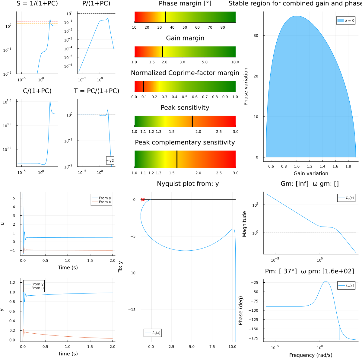
Analysis Arguments
The following arguments define a ClosedLoopAnalysis:
Required Arguments
model: The model to be analyzed.measurement::Vector{String}: Name of the measurement signal analysis points (plant outputs).control_input::Vector{String}: Name of the control input signal analysis points.
Optional Arguments
loop_openings::Vector{String} = String[]: Names of additional analysis points at which the loop is opened during linearization (e.g. the reference input"r").wl::Real = -1: Lower frequency bound for analysis (set to -1 for automatic selection).wu::Real = -1: Upper frequency bound for analysis (set to -1 for automatic selection).num_frequencies::Int = 300: Number of frequency points.t::Real = 0.0: Time at which the model is linearized for the analysis.pos_feedback::Bool = true: Whether the feedback is positive (default is true; negative feedback is often built into the model).duration::Real = -1.0: Duration of the step-response simulation (set to -1 for automatic selection).
Artifacts
A ClosedLoopAnalysis returns the following artifacts:
Standard Plots
all: Combined plot showing:Bode plots of
, , Disk margin and classical margins
Step responses to reference and disturbance steps
Further Reading
Notes about MIMO Systems
When MIMO systems are analyzed, some sensitivity functions are drawn as Sigma plots rather than Bode plots. The disk margin is in this case computed for the output loop-transfer function