MPC with quadratic cost functions
This tutorial demonstrates an MPC controller with a quadratic cost function for a nonlinear system, using the component ACADOSMPC. The optimization problem is solved using sequential quadratic programming (SQP). The formulation supports nonlinear dynamics, quadratic cost functions and bound constraints on control and state variables.
A video tutorial on quadratic MPC with the DyadControlSystems implementation, which differs from the one used here, is available in the form of a webinar:
Getting started: Nonlinear system
We begin the exposition of the MPC functionality with an example.
In this example, we will design an MPC controller for a pendulum on a cart. We start by defining the dynamics, here as the Dyad component CartPolePlant, which is also available as MPCComponents.Examples.CartPolePlant. The state is
corresponding to position, angle, velocity and angular velocity. The angle F acting on the cart.
"""
Cart-pole: a cart of mass `mc` driven by the force `F`, carrying a pendulum of mass `mp` and length `l`.
The angle `theta` is zero when the pendulum hangs down. Translated from the DyadControlSystems
quadratic-MPC tutorial.
"""
component CartPolePlant
  "Force on the cart"
  F = RealInput() {^F}
  "Cart position"
  pos = RealOutput() {^pos}
  "Pendulum angle"
  theta = RealOutput() {^theta}
  "Cart velocity"
  vel = RealOutput() {^vel}
  "Pendulum angular velocity"
  omega = RealOutput() {^omega}
  parameter mc::Real = 1.0
  parameter mp::Real = 0.2
  parameter l::Real = 0.5
  parameter g::Real = 9.81
  parameter p0::Real = 0.0
  parameter th0::Real = 0.0
  parameter v0::Real = 0.0
  parameter w0::Real = 0.0
  variable p::Real
  variable th::Real
  variable v::Real
  variable w::Real
relations
  initial p = p0
  initial th = th0
  initial v = v0
  initial w = w0
  der(p) = v
  der(th) = w
  der(v) = (F + mp * l * sin(th) * w ^ 2 + mp * g * sin(th) * cos(th)) / (mc + mp * sin(th) ^ 2)
  der(w) = -(cos(th) * (F + mp * l * sin(th) * w ^ 2) + (mc + mp) * g * sin(th)) / (l * (mc + mp * sin(th) ^ 2))
  pos = p
  theta = th
  vel = v
  omega = w
metadata {
  "Dyad": {
    "icons": {"default": "dyad://MPCComponents/CartPolePlant.svg"},
    "doc": {"behavior": false}
  },
  "_links": {
    "F": {
      "Dyad": {"placement": {"diagram": {"x1": -100, "x2": 0, "y1": 450, "y2": 550}}}
    },
    "pos": {
      "Dyad": {"placement": {"diagram": {"x1": 1000, "x2": 1100, "y1": 100, "y2": 200}}}
    },
    "theta": {
      "Dyad": {"placement": {"diagram": {"x1": 1000, "x2": 1100, "y1": 330, "y2": 430}}}
    },
    "vel": {
      "Dyad": {"placement": {"diagram": {"x1": 1000, "x2": 1100, "y1": 610, "y2": 710}}}
    },
    "omega": {
      "Dyad": {"placement": {"diagram": {"x1": 1000, "x2": 1100, "y1": 830, "y2": 930}}}
    }
  }
}
end
We also define some problem parameters. The system has one control input, the state dimension is 4, and all state components are measured. The sample time is Ts = 0.02, which is both the period of the clock that triggers the controller and the parameter Ts of the controller, and the MPC optimization horizon is Np = 15 shooting intervals (the control horizon is also equal to Np). The initial state has the cart at position 3 and the pendulum at the angle p0 and th0, and the reference state is the origin, which the controller regulates to when reference_tracking = false:
periodicclock = DiscreteComponents.PeriodicClock(dt = 0.02)
plant = CartPolePlant(p0 = 3.0, th0 = 1.5707963267948966)
mpc = MPCComponents.ACADOSMPC(dynamics = plant,
                              inputs = ["F"],
                              state_variables = ["p", "th", "v", "w"],
                              outputs = ["p", "th", "v", "w"],
                              Ts = 0.02,
                              Np = Np,
                              reference_tracking = reference_tracking,
                              ...)
Here, Np and reference_tracking are parameters of the closed-loop model below, with the default values 15 and false.
Next, we specify the discretization of the dynamics and the cost-function matrices. The controller discretizes the prediction model itself: acados integrates the continuous-time dynamics over each shooting interval with its default integrator, the explicit Runge-Kutta method with 4 stages (integrator = ERK, integrator_stages = 4), i.e., one RK4 step per interval. Since the full state is measured, the controlled outputs outputs are the four state variables, and the state cost matrix Q1 weighs all of them. The control cost matrix Q2 equals Ts (a penalty on the control derivative is also supported, through penalize_increments and Q3). The control is limited to constrained is left empty; state constraints are soft by default when enabled):
structural parameter Q1::Real[4, 4] = diagonal([1.0, 1.0, 1.0, 1.0])Q1 = Q1,
Q2 = diagonal([0.02]),
umin = [-5.0],
umax = [5.0],The weights are matrices, and diagonal constructs a diagonal matrix from a vector.
The four Sampler components feed the state of the plant to the controller, i.e., the controller operates with state feedback. acados solves the optimization problem with one SQP iteration per sample (real-time iteration, nlp_solver = SQP_RTI), starting from the solution of the previous sample shifted by one step, and each quadratic subproblem is solved by HPIPM. A Levenberg-Marquardt regularization is added to the Gauss-Newton approximation of the Hessian:
levenberg_marquardt = 1.0,
nlp_solver = MPCComponents.ACADOSSolver.SQP_RTI()
Our dynamics is nonlinear, but our cost is quadratic, and we complement the quadratic stage cost with a quadratic terminal cost given by the solution to the discrete-time algebraic Riccati equation: terminal_lqr_cost = true uses the infinite-horizon LQR cost of the model linearized at the origin as terminal weight on the full state, instead of Qf.
terminal_lqr_cost = terminal_lqr_cost,In the closed-loop model, terminal_lqr_cost defaults to !reference_tracking, i.e., to true. Without this terminal cost, the prediction horizon of
With the controller configured, we assemble the closed-loop model: the PeriodicClock determines the sample instants, the samplers s convert the continuous-time state of the plant into the discrete-time controller input x, and the zero-order hold zoh holds the force between samples. The variables pos, theta, u1 and flag make the signals of interest available for plotting, flag being the acados status of each solve (0 indicates success). The optional reference input angle_ref is present only when reference_tracking = true.
"""
Cart-pole regulation with `ACADOSMPC`: from the cart at position 3 with the pendulum horizontal
(θ = π/2), bring the cart to the origin with the pendulum hanging at rest, with the force bounded to
±5. Translated from the DyadControlSystems quadratic-MPC tutorial (Ts = 0.02, N = 15, Q1 = I,
Q2 = Ts). The terminal weight is the LQR cost of the linearized model (`terminal_lqr_cost = true`),
which the tutorial's `QMPCProblem` adds implicitly.
"""
example component CartPoleMPCExample
  periodicclock = DiscreteComponents.PeriodicClock(dt = 0.02) {^periodicclock}
  plant = CartPolePlant(p0 = 3.0, th0 = 1.5707963267948966) {^plant}
  "Samplers of the four state variables"
  s = [DiscreteComponents.Sampler() for i in 1:4] {^s}
  zoh = DiscreteComponents.ZeroOrderHold() {^zoh}
  mpc = MPCComponents.ACADOSMPC(dynamics = plant, inputs = ["F"], state_variables = ["p", "th", "v", "w"], outputs = ["p", "th", "v", "w"], Ts = 0.02, Np = Np, Q1 = Q1, Q2 = diagonal([0.02]), terminal_lqr_cost = terminal_lqr_cost, umin = [-5.0], umax = [5.0], reference_tracking = reference_tracking, levenberg_marquardt = 1.0, nlp_solver = MPCComponents.ACADOSSolver.SQP_RTI()) {^mpc}
  angle_ref = BlockComponents.Sources.Constant(k = k) if reference_tracking {^angle_ref}
  "Cart position"
  variable pos::Real
  "Pendulum angle"
  variable theta::Real
  "Force"
  variable u1::Real
  "acados status"
  variable flag::Real
  "The constant value to output"
  parameter k::Real = 0
  "Prediction horizon (number of shooting intervals)"
  structural parameter Np::Integer = 15
  "Use the infinite-horizon LQR cost of the model linearized at the origin as terminal weight (on the full state) instead of Qf; requires reference_tracking = false. In Julia the weight follows Q1 and Q2; in exported C it stays at its export-time value"
  structural parameter terminal_lqr_cost::Boolean = !reference_tracking
  "Track references (adds the r input); false regulates to the origin"
  structural parameter reference_tracking::Boolean = false
  "Output weight on C*x - r (ny × ny, e.g. diagonal([1.0, 10.0])); tunable. Default: the identity, or the weight the mpc object was built with"
  structural parameter Q1::Real[4, 4] = diagonal([1.0, 1.0, 1.0, 1.0])
relations
  pos = plant.pos
  theta = plant.theta
  u1 = mpc.u[1]
  flag = mpc.exitflag
  connect(plant.pos, s[1].u) {^id7}
  connect(plant.theta, s[2].u) {^id8}
  connect(plant.vel, s[3].u) {^id9}
  connect(plant.omega, s[4].u) {^id10}
  connect(s[1].y, mpc.x[1], periodicclock.y) {^id11}
  for i in 2:4
    connect(s[i].y, mpc.x[i])
  end
  connect(mpc.u[1], zoh.u) {^id12}
  connect(zoh.y, plant.F) {^id13}
  if reference_tracking
    connect(angle_ref.y, mpc.r[2]) {^id14}
    mpc.r[1] = 0
    mpc.r[3] = 0
    mpc.r[4] = 0
  end
metadata {
  "Dyad": {"doc": {"behavior": false}},
  "_links": {
    "periodicclock": {
      "Dyad": {"placement": {"diagram": {"x1": 465, "x2": 565, "y1": 43, "y2": 143}}}
    },
    "plant": {
      "Dyad": {"placement": {"diagram": {"x1": 40, "x2": 140, "y1": 140, "y2": 240}}}
    },
    "s": {
      "Dyad": {"placement": {"diagram": {"x1": 194, "x2": 294, "y1": 140, "y2": 240}}}
    },
    "zoh": {
      "Dyad": {"placement": {"diagram": {"x1": 464, "x2": 564, "y1": 163, "y2": 263}}}
    },
    "mpc": {
      "Dyad": {"placement": {"diagram": {"x1": 330, "x2": 430, "y1": 140, "y2": 240}}}
    },
    "angle_ref": {"Dyad": {"placement": {"diagram": {"x1": 40, "x2": 140, "y1": -90, "y2": 10}}}},
    "id7": {
      "Dyad": {
        "edges": [{"S": 1, "M": [{"x": 170, "y": 155}, {"x": 170, "y": 190}], "E": 2}],
        "path": {}
      }
    },
    "id8": {
      "Dyad": {
        "edges": [{"S": 1, "M": [{"x": 170, "y": 178}, {"x": 170, "y": 190}], "E": 2}],
        "path": {}
      }
    },
    "id9": {"Dyad": {"edges": [{"S": 1, "M": [{"x": 145, "y": 190}], "E": 2}], "path": {}}},
    "id10": {
      "Dyad": {
        "edges": [{"S": 1, "M": [{"x": 170, "y": 228}, {"x": 170, "y": 190}], "E": 2}],
        "path": {}
      }
    },
    "id11": {
      "Dyad": {
        "edges": [
          {"S": 1, "M": [], "E": 2},
          {"S": 2, "M": [{"x": 310, "y": 190}, {"x": 310, "y": 93}], "E": 3}
        ],
        "path": {}
      }
    },
    "id12": {"Dyad": {"edges": [{"S": 1, "M": [], "E": 2}], "path": {}}},
    "id13": {
      "Dyad": {
        "edges": [
          {
            "S": 1,
            "M": [
              {"x": 580, "y": 213},
              {"x": 580, "y": 300},
              {"x": 20, "y": 300},
              {"x": 20, "y": 190}
            ],
            "E": 2
          }
        ],
        "path": {}
      }
    },
    "id14": {
      "Dyad": {
        "edges": [{"S": 1, "M": [{"x": 320, "y": -40}, {"x": 320, "y": 155}], "E": 2}],
        "path": {}
      }
    }
  }
}
end
We instantiate the model in Julia and compile it. Models that contain clocked (discrete-time) components, such as the controller, are compiled with the additional pass SynchToolkit.compile_lustre, which compiles the discrete-time partitions of the model.
@named model = CartPoleMPCExample()
ssys = mtkcompile(model; additional_passes = [SynchToolkit.compile_lustre])
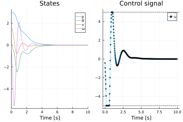
We may now run the MPC controller in closed loop with the plant for 500 time steps, i.e., 10 s:
prob = ODEProblem(ssys, [], (0.0, 10.0))
sol = solve(prob)plot(sol, idxs = [ssys.plant.p, ssys.plant.th, ssys.plant.v, ssys.plant.w], layout = (1, 2), sp = 1, title = "States", lab = ["p" "θ" "v" "ω"], xlabel = "Time [s]")
plot!(sol, idxs = [ssys.u1], sp = 2, title = "Control signal", lab = "u", xlabel = "Time [s]")
hline!([-5.0 5.0], sp = 2, l = (:black, :dash), lab = "")