LIBRARY

Math.Tests.Acos
Computes the arc cosine of constant and time-varying inputs.
Connects a constant source with value 1 to an Acos block and verifies that acos(1) = 0.
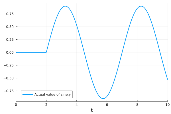
Connects a sine source (amplitude 0.9, frequency 1/5, starting at t = 2) to a second Acos block. The input stays within the valid domain [-1, 1] while sweeping negative and positive values, exercising the arc cosine over its full output range [0, π].
Usage
BlockComponents.Math.Tests.Acos()
Behavior
Source
dyad
"""
Computes the arc cosine of constant and time-varying inputs.

Connects a constant source with value 1 to an Acos block and verifies that
acos(1) = 0.

Connects a sine source (amplitude 0.9, frequency 1/5, starting at t = 2) to a
second Acos block. The input stays within the valid domain [-1, 1] while
sweeping negative and positive values, exercising the arc cosine over its full
output range [0, π].
"""
test component Acos
  "Constant source providing the input value"
  c1 = BlockComponents.Sources.Constant(k = 1) {
    "Dyad": {
      "placement": {
        "diagram": {"iconName": "default", "x1": 20, "y1": 20, "x2": 120, "y2": 120, "rot": 0}
      },
      "tags": []
    }
  }
  "Sine source sweeping the valid input domain"
  sine = BlockComponents.Sources.Sine(start_time = 2, amplitude = 0.9, frequency = 1 / 5) {
    "Dyad": {
      "placement": {
        "diagram": {"iconName": "default", "x1": 20, "y1": 190, "x2": 120, "y2": 290, "rot": 0}
      },
      "tags": []
    }
  }
  "Acos block under test"
  acos_block_1 = BlockComponents.Math.Acos() {
    "Dyad": {
      "placement": {
        "diagram": {"iconName": "default", "x1": 170, "y1": 20, "x2": 270, "y2": 120, "rot": 0}
      },
      "tags": []
    }
  }
  "Second Acos block under test"
  acos_block_2 = BlockComponents.Math.Acos() {
    "Dyad": {
      "placement": {
        "diagram": {"iconName": "default", "x1": 170, "y1": 190, "x2": 270, "y2": 290, "rot": 0}
      },
      "tags": []
    }
  }
relations
  connect(c1.y, acos_block_1.u) {"Dyad": {"edges": [{"S": 1, "M": [], "E": 2}], "renderStyle": "standard"}}
  connect(sine.y, acos_block_2.u) {"Dyad": {"edges": [{"S": 1, "M": [], "E": 2}], "renderStyle": "standard"}}
metadata {
  "Dyad": {
    "icons": {"default": "dyad://BlockComponents/Example.svg"},
    "tests": {
      "case1": {
        "stop": 10,
        "expect": {"signals": ["acos_block_1.y", "acos_block_2.y", "sine.y"]}
      }
    }
  }
}
end
Flattened Source
dyad
"""
Computes the arc cosine of constant and time-varying inputs.

Connects a constant source with value 1 to an Acos block and verifies that
acos(1) = 0.

Connects a sine source (amplitude 0.9, frequency 1/5, starting at t = 2) to a
second Acos block. The input stays within the valid domain [-1, 1] while
sweeping negative and positive values, exercising the arc cosine over its full
output range [0, π].
"""
test component Acos
  "Constant source providing the input value"
  c1 = BlockComponents.Sources.Constant(k = 1) {
    "Dyad": {
      "placement": {
        "diagram": {"iconName": "default", "x1": 20, "y1": 20, "x2": 120, "y2": 120, "rot": 0}
      },
      "tags": []
    }
  }
  "Sine source sweeping the valid input domain"
  sine = BlockComponents.Sources.Sine(start_time = 2, amplitude = 0.9, frequency = 1 / 5) {
    "Dyad": {
      "placement": {
        "diagram": {"iconName": "default", "x1": 20, "y1": 190, "x2": 120, "y2": 290, "rot": 0}
      },
      "tags": []
    }
  }
  "Acos block under test"
  acos_block_1 = BlockComponents.Math.Acos() {
    "Dyad": {
      "placement": {
        "diagram": {"iconName": "default", "x1": 170, "y1": 20, "x2": 270, "y2": 120, "rot": 0}
      },
      "tags": []
    }
  }
  "Second Acos block under test"
  acos_block_2 = BlockComponents.Math.Acos() {
    "Dyad": {
      "placement": {
        "diagram": {"iconName": "default", "x1": 170, "y1": 190, "x2": 270, "y2": 290, "rot": 0}
      },
      "tags": []
    }
  }
relations
  connect(c1.y, acos_block_1.u) {"Dyad": {"edges": [{"S": 1, "M": [], "E": 2}], "renderStyle": "standard"}}
  connect(sine.y, acos_block_2.u) {"Dyad": {"edges": [{"S": 1, "M": [], "E": 2}], "renderStyle": "standard"}}
metadata {
  "Dyad": {
    "icons": {"default": "dyad://BlockComponents/Example.svg"},
    "tests": {
      "case1": {
        "stop": 10,
        "expect": {"signals": ["acos_block_1.y", "acos_block_2.y", "sine.y"]}
      }
    }
  }
}
end
Test Cases
Test Case case1
julia
plt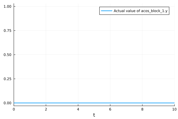
julia
plt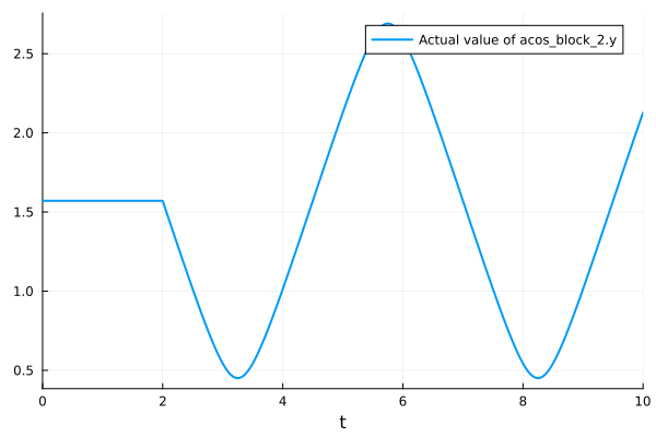
julia
plt