
Closed-Loop Sensitivity Analysis
Download as a Dyad projectClosedLoopSensitivityExample.zipOpen in Dyad Studio
The Closed-Loop Sensitivity Analysis computes and visualizes the sensitivity function
Method Overview
The sensitivity function
         ▲
         │e₁
         │  ┌─────┐
d₁────+──┴──►  P  ├─────┬──►e₄
      │     └─────┘    y│
      │u                │
      │     ┌─────┐    -│
 e₂◄──┴─────┤  C  ◄──┬──+───d₂
            └─────┘  │
                     │e₃
                     ▼
performing a sensitivity analysis at the analysis point y computes the output sensitivity function u computes the input sensitivity function
This analysis linearizes the model and computes the sensitivity function at the specified analysis point or points, optionally breaking feedback loops as needed.
The peak value of
Example Definition
This example is a continuation of the DC Motor Control tutorial. We will analyze the sensitivity function y.
We set w_motor to zero so the controller does not saturate at the linearization point. Since the analysis opens the loop at r, the connection to controller.u_s is broken during linearization. We provide an initial condition so the operating point is well-defined:
using DyadInterface: artifacts
using Plots
asol = DCMotorClosedLoopSensitivityAnalysis()
ClosedLoopSensitivityAnalysisSolution
Analysis points: ["y"]
Loop openings: ["r"]
Frequency bounds: [1.0, 10000.0]
H∞ norm ||S(s)||: 1.9
Phase margin lower bound: 31.0°
Gain margin lower bound: 2.1fig = artifacts(asol, :BodePlot)
plot!(legend = :bottomright)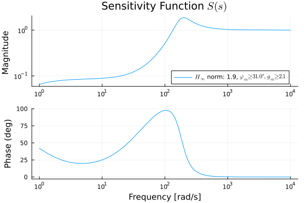
Analysis Arguments
The following arguments define a ClosedLoopSensitivityAnalysis:
Required Arguments
model: The model to be analyzed.analysis_points::Vector{String}: Name of the analysis points where sensitivity is computed.
Optional Arguments
loop_openings::Vector{String} = []: Names of loop openings to break feedback if present.wl::Real = -1.0: Lower frequency bound for the analysis (set to -1 for automatic selection).wu::Real = -1.0: Upper frequency bound for the analysis (set to -1 for automatic selection).
Artifacts
A ClosedLoopSensitivityAnalysis returns the following artifact:
Standard Plot
BodePlot: Bode plot of the closed-loop sensitivity function. The plot includes the norm (maximum value), and the corresponding minimum gain and phase margins. For MIMO analysis, the plot shows the singular values of the sensitivity function as a function of frequency.