
Control design for a quadruple-tank system
In this example, we will implement two controllers for a nonlinear MIMO process, a linear MPC controller and a nonlinear MPC controller, both with state and input constraints.
The DyadControlSystems version of this example, which covers additional controllers, has an associated video where we provide additional context and insights:
The process we will consider is a quadruple tank, where two upper tanks feed into two lower tanks, depicted in the schematics below. The quad-tank process is a well-studied example in many multivariable control courses, this particular instance of the process is borrowed from the Lund University introductory course on automatic control.
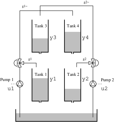
The process has a cross coupling between the tanks, governed by the parameters
The dynamics are given by
where
In the examples below, the levels of all four tanks are measured. The nonlinear MPC controller receives the sampled levels directly, while the linear MPC controller estimates its state with a Kalman filter.
The interested reader can find more details on the quadruple-tank process from the manual provided here (see "lab 2"), from where the example is taken.
We will consider two variants of the MPC controller:
Linear MPC with a linear observer and prediction model.
Nonlinear MPC using the nonlinear model of the process for prediction.
The DyadControlSystems version of this example additionally covers a PID controller, a linear MPC controller with a nonlinear observer, and a linear MPC controller with integral action and robust tuning, which are not covered here.
In all cases we will consider constraints on the control authority of the pumps as well as the levels of the tanks.
We start by defining the dynamics. All four tanks have the same cross-sectional area A and outlet area a, and the square roots are regularized so that the model is smooth near empty tanks:
"""
Quadruple-tank process (Johansson) with two pumps: the lower tanks 1 and 2 are fed by their own pump
and by the tank above; the fraction of each pump flow reaching the lower tank is `gamma`. Levels in cm,
pump voltages in V. Translated from the DyadControlSystems quadtank tutorial (non-minimum-phase setting
`gamma1 = gamma2 = 0.2`). The square roots are regularized so the model is smooth near empty tanks.
"""
component QuadTankPlant
  "Pump 1 voltage"
  u1 = RealInput() {^u1}
  "Pump 2 voltage"
  u2 = RealInput() {^u2}
  "Level of tank 1"
  y1 = RealOutput() {^y1}
  "Level of tank 2"
  y2 = RealOutput() {^y2}
  "Level of tank 3"
  y3 = RealOutput() {^y3}
  "Level of tank 4"
  y4 = RealOutput() {^y4}
  parameter k1::Real = 1.6
  parameter k2::Real = 1.6
  parameter g::Real = 9.81
  parameter A::Real = 4.9
  parameter a::Real = 0.03
  parameter gamma1::Real = 0.2
  parameter gamma2::Real = 0.2
  "Initial levels"
  parameter h10::Real = 2.0
  parameter h20::Real = 1.0
  parameter h30::Real = 8.0
  parameter h40::Real = 3.0
  variable h1::Real(initial = h10)
  variable h2::Real(initial = h20)
  variable h3::Real(initial = h30)
  variable h4::Real(initial = h40)
relations
  der(h1) = -a / A * sqrt(max(2 * g * h1, 0) + 0.001) + a / A * sqrt(max(2 * g * h3, 0) + 0.001) + gamma1 * k1 / A * u1
  der(h2) = -a / A * sqrt(max(2 * g * h2, 0) + 0.001) + a / A * sqrt(max(2 * g * h4, 0) + 0.001) + gamma2 * k2 / A * u2
  der(h3) = -a / A * sqrt(max(2 * g * h3, 0) + 0.001) + (1 - gamma2) * k2 / A * u2
  der(h4) = -a / A * sqrt(max(2 * g * h4, 0) + 0.001) + (1 - gamma1) * k1 / A * u1
  y1 = h1
  y2 = h2
  y3 = h3
  y4 = h4
metadata {
  "Dyad": {
    "icons": {"default": "dyad://MPCComponents/QuadTankPlant.svg"},
    "doc": {"behavior": false}
  },
  "_links": {
    "u1": {
      "Dyad": {"placement": {"diagram": {"x1": -100, "x2": 0, "y1": 210, "y2": 310}}}
    },
    "u2": {
      "Dyad": {"placement": {"diagram": {"x1": -100, "x2": 0, "y1": 730, "y2": 830}}}
    },
    "y1": {
      "Dyad": {"placement": {"diagram": {"x1": 1000, "x2": 1100, "y1": 110, "y2": 210}}}
    },
    "y2": {
      "Dyad": {"placement": {"diagram": {"x1": 1000, "x2": 1100, "y1": 320, "y2": 420}}}
    },
    "y3": {
      "Dyad": {"placement": {"diagram": {"x1": 1000, "x2": 1100, "y1": 580, "y2": 680}}}
    },
    "y4": {
      "Dyad": {"placement": {"diagram": {"x1": 1000, "x2": 1100, "y1": 800, "y2": 900}}}
    }
  }
}
end
The initial levels of the tanks are given by the parameters h10, h20, h30 and h40, i.e.,
Next, we define the constraints and an operating point. We start by defining a desired state at the operating point,
xr = [9.818427, 9.818427, 6.283709, 6.283709] # stationary levels
ur = [0.260238, 0.260238] # pump voltages at the stationary point
The pump voltages are limited to
umin = [0.0, 0.0],
umax = [0.6, 0.6],
ymin = [0.0, 0.0, 0.0, 0.0],
ymax = [12.0, 12.0, 8.0, 8.0],
and
umin = [0.0, 0.0],
umax = [0.6, 0.6],
constrained = ["h1", "h2", "h3", "h4"],
constrained_min = [0.0, 0.0, 0.0, 0.0],
constrained_max = [12.0, 12.0, 8.0, 8.0],
The input constraints are hard, while the level constraints are soft by default in both controllers.
Linear MPC
With a MPC controller, we can take the constraints into account explicitly in the optimization problem solved at each sample time.
In some situations, we may want to resort to a linear MPC controller. A linear controller is often sufficient when the task is regulation, i.e., keeping a controlled variable at a fixed set point.
We make use of the model linearized around the operating point
For a linear MPC controller to work well, we must provide the operating point around which we linearize. The controller LinearMPCController takes the plant as its prediction model (dynamics = plant_lin) and linearizes it itself: linearization_point = SteadyState() selects the steady state of the plant at the pump voltages u_op, which is the operating point state_variables names the levels that define the state coordinates. The continuous-time linearization in the affine form Ts, and the offset carries the operating point, so that the controller operates on the levels themselves rather than on deviations from the operating point. The controller also contains a Kalman filter for state estimation, designed from the dynamics covariance R1 and the measurement covariance R2, with the initial state estimate x0:
dynamics = plant_lin,
inputs = ["u1", "u2"],
outputs = ["y1", "y2", "y3", "y4"],
state_variables = ["h1", "h2", "h3", "h4"],
linearization_point = MPCComponents.LinearizationPoint.SteadyState(),
u_op = [0.260238, 0.260238],
Ts = 2.0,
R1 = [0.00001, 0.00001, 0.00001, 0.00001],
R2 = [1.0, 1.0, 1.0, 1.0],
x0 = [2.0, 1.0, 8.0, 3.0],
We also specify some cost matrices for the MPC problem and the prediction horizon Q1 weights the deviation of the levels from the reference, Q3 the control increments Q2 is a small penalty on the control signal itself. A penalty on the control signal leaves a steady-state error in proportion to its weight, which is why this weight is small.
Np = 10,
Q1 = [1.0, 1.0, 1.0, 1.0],
Q2 = [0.0001, 0.0001],
Q3 = [1.0, 1.0],
The closed-loop model below contains both controllers, each connected to its own instance of the plant, so that one simulation yields the results of both designs; the nonlinear controller mpc_nl is discussed in the section on nonlinear MPC below. A PeriodicClock with period Ts determines the sample instants, the samplers s and sl sample the levels of the two plants, the samplers sr sample the references, which are the levels at the operating point, and the zero-order holds zoh and zohl hold the pump voltages between samples. The variables h1_nl, h1_lin, u1_nl, u1_lin and flag make signals of interest available for plotting, flag being the acados status of each solve of the nonlinear controller (0 indicates success).
"""
Quadruple-tank level control: the same plant under a linear MPC (`LinearMPCController` on the
linearization at the operating point, with a Kalman filter and a control-increment penalty, as in the
tutorial's linear MPC) and under a nonlinear MPC (`ACADOSMPC` with the plant itself as the prediction
model), both driving the levels from [2, 1, 8, 3] to the operating point [9.82, 9.82, 6.28, 6.28] with
the pump voltages in [0, 0.6] and the levels softly bounded by [12, 12, 8, 8]. Translated from the
DyadControlSystems quadtank tutorial.
"""
example component QuadTankMPCExample
  periodicclock = DiscreteComponents.PeriodicClock(dt = 2.0) {^periodicclock}
  plant_nl = QuadTankPlant() {^plant_nl}
  plant_lin = QuadTankPlant() {^plant_lin}
  "Level samplers of the nonlinear loop"
  s = [DiscreteComponents.Sampler() for i in 1:4] {^s}
  "Level samplers of the linear loop"
  sl = [DiscreteComponents.Sampler() for i in 1:4] {^sl}
  "Pump voltage holds of the nonlinear loop"
  zoh = [DiscreteComponents.ZeroOrderHold() for i in 1:2] {^zoh}
  "Pump voltage holds of the linear loop"
  zohl = [DiscreteComponents.ZeroOrderHold() for i in 1:2] {^zohl}
  "Level reference of the lower tanks 1 and 2"
  r_lower = BlockComponents.Sources.Constant(k = 9.818427) {^r_lower}
  "Level reference of the upper tanks 3 and 4"
  r_upper = BlockComponents.Sources.Constant(k = 6.283709) {^r_upper}
  "Reference samplers"
  sr = [DiscreteComponents.Sampler() for i in 1:4] {^sr}
  mpc_nl = MPCComponents.ACADOSMPC(dynamics = plant_nl, inputs = ["u1", "u2"], state_variables = ["h1", "h2", "h3", "h4"], outputs = ["h1", "h2", "h3", "h4"], Ts = 2.0, Np = 10, Q1 = diagonal([1.0, 1.0, 1.0, 1.0]), Q2 = diagonal([1.0, 1.0]), umin = [0.0, 0.0], umax = [0.6, 0.6], constrained = ["h1", "h2", "h3", "h4"], constrained_min = [0.0, 0.0, 0.0, 0.0], constrained_max = [12.0, 12.0, 8.0, 8.0]) {^mpc_nl}
  mpc_lin = MPCComponents.LinearMPCController(dynamics = plant_lin, inputs = ["u1", "u2"], outputs = ["y1", "y2", "y3", "y4"], state_variables = ["h1", "h2", "h3", "h4"], linearization_point = MPCComponents.LinearizationPoint.SteadyState(), u_op = [0.260238, 0.260238], Ts = 2.0, Np = 10, Q1 = [1.0, 1.0, 1.0, 1.0], Q2 = [0.0001, 0.0001], Q3 = [1.0, 1.0], umin = [0.0, 0.0], umax = [0.6, 0.6], ymin = [0.0, 0.0, 0.0, 0.0], ymax = [12.0, 12.0, 8.0, 8.0], R1 = [0.00001, 0.00001, 0.00001, 0.00001], R2 = [1.0, 1.0, 1.0, 1.0], x0 = [2.0, 1.0, 8.0, 3.0]) {^mpc_lin}
  "Tank 1 level, nonlinear MPC"
  variable h1_nl::Real
  "Tank 1 level, linear MPC"
  variable h1_lin::Real
  "Pump 1 voltage, nonlinear MPC"
  variable u1_nl::Real
  "Pump 1 voltage, linear MPC"
  variable u1_lin::Real
  "acados status"
  variable flag::Real
relations
  h1_nl = plant_nl.y1
  h1_lin = plant_lin.y1
  u1_nl = mpc_nl.u[1]
  u1_lin = mpc_lin.u[1]
  flag = mpc_nl.exitflag
  connect(plant_nl.y1, s[1].u)
  connect(plant_nl.y2, s[2].u)
  connect(plant_nl.y3, s[3].u)
  connect(plant_nl.y4, s[4].u)
  connect(s[1].y, mpc_nl.x[1], periodicclock.y)

  connect(s[2].y, mpc_nl.x[2])
  connect(s[3].y, mpc_nl.x[3])
  connect(s[4].y, mpc_nl.x[4])
  connect(r_lower.y, sr[1].u, sr[2].u)
  connect(r_upper.y, sr[3].u, sr[4].u)
  # Connected entry by entry only because the compiler lowers a connect of a component array to a
  # field access on the array (JuliaComputing/dyad-lang#2247). Connections in loops are not shown in
  # the diagram, so restore the array connections connect(sr.y, mpc_nl.r, mpc_lin.r),
  # connect(mpc_nl.u, zoh.u), connect(mpc_lin.u, zohl.u) and connect(sl.y, mpc_lin.y) once it is fixed
  for i in 1:4
    connect(sr[i].y, mpc_nl.r[i], mpc_lin.r[i])
  end

  for i in 1:2
    connect(mpc_nl.u[i], zoh[i].u)
    connect(mpc_lin.u[i], zohl[i].u)
  end
  connect(zoh[1].y, plant_nl.u1)
  connect(zoh[2].y, plant_nl.u2)
  connect(plant_lin.y1, sl[1].u)
  connect(plant_lin.y2, sl[2].u)
  connect(plant_lin.y3, sl[3].u)
  connect(plant_lin.y4, sl[4].u)
  for i in 1:4
    connect(sl[i].y, mpc_lin.y[i])
  end
  connect(zohl[1].y, plant_lin.u1)
  connect(zohl[2].y, plant_lin.u2)
metadata {
  "Dyad": {"doc": {"behavior": false}},
  "_links": {
    "periodicclock": {},
    "plant_nl": {},
    "plant_lin": {},
    "s": {},
    "sl": {},
    "zoh": {},
    "zohl": {},
    "r_lower": {},
    "r_upper": {},
    "sr": {},
    "mpc_nl": {},
    "mpc_lin": {}
  }
}
end
We instantiate the model in Julia and compile it. Models that contain clocked (discrete-time) components, such as the controllers, are compiled with the additional pass SynchToolkit.compile_lustre, which compiles the discrete-time partitions of the model.
@named model = QuadTankMPCExample()
ssys = mtkcompile(model; additional_passes = [SynchToolkit.compile_lustre])
We now simulate the linear MPC:
prob = ODEProblem(ssys, [], (0.0, 1000.0))
sol = solve(prob)
plot(sol, idxs = [ssys.plant_lin.h1, ssys.plant_lin.h2, ssys.plant_lin.h3, ssys.plant_lin.h4], layout = (1, 2), sp = 1,
     title = "States", lab = ["h1" "h2" "h3" "h4"], plot_title = "Linear MPC", legend = :bottomright, xlabel = "Time [s]")
hline!(xr', sp = 1, l = :dash, c = (1:4)', lab = "")
plot!(sol, idxs = [ssys.mpc_lin.u[1], ssys.mpc_lin.u[2]], sp = 2, title = "Control signal", lab = ["u1" "u2"], xlabel = "Time [s]", ms = 2, msw = 0)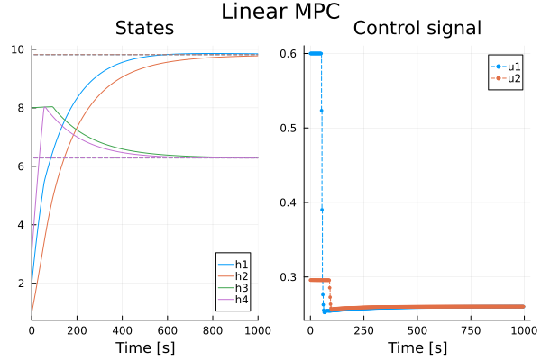
The controller performs reasonably well and respects the input constraints. Pump 1 operates at its upper bound during the first part of the transient, and while the level of tank 3 is at its upper bound, the controller holds the voltage of pump 2, which feeds tank 3, at a lower level.
With a linear observer, we notice a slight violation of the state constraints for states R1 is small compared to the measurement covariance R2, so the estimate of the observer relies mostly on the linear model. Due to the square root in the dynamics that govern the outflow of liquid from the tanks, the observer estimates the outflow to be greater than it actually is at levels well above the linearization point, and the estimated level of tank 3 remains at the bound while the actual level exceeds it.
In practice, it is unrealistic to assume that we know the static gain of the system perfectly, in fact, the static gain for this system probably varies with the temperature of the equipment, the tank contents and during the lifetime of the tanks and pumps. We would thus likely end up with a stationary error using the controller above. This highlights a problem with naive MPC control (and similarly for standard LQG control), we do not have any integral action in the controller! LinearMPCController provides integral action through an offset-free observer, selected with the parameter offset_free, see the example LinearMPCOffsetFreeExample.
Nonlinear MPC
The last controller we will consider is a nonlinear MPC controller that uses the nonlinear model of the plant for prediction, the component ACADOSMPC. The prediction model is the plant plant_nl itself, and since the controller receives the four sampled levels, it does not require an observer. The weights are Q1 = I on the deviation of the levels from the reference and Q2 = I on the pump voltages, and the constraints are the ones given above. The DyadControlSystems version penalizes the deviation of the pump voltages from their values at the operating point, whereas Q2 here penalizes the pump voltages themselves:
mpc_nl = MPCComponents.ACADOSMPC(dynamics = plant_nl,
                                 inputs = ["u1", "u2"],
                                 state_variables = ["h1", "h2", "h3", "h4"],
                                 outputs = ["h1", "h2", "h3", "h4"],
                                 Ts = 2.0,
                                 Np = 10,
                                 Q1 = diagonal([1.0, 1.0, 1.0, 1.0]),
                                 Q2 = diagonal([1.0, 1.0]),
                                 ...)
The optimization problems are solved by acados using sequential quadratic programming, and the prediction model is integrated with an explicit Runge-Kutta scheme (the default integrator). The solution computed above contains the nonlinear loop as well:
plot(sol, idxs = [ssys.plant_nl.h1, ssys.plant_nl.h2, ssys.plant_nl.h3, ssys.plant_nl.h4], layout = (1, 2), sp = 1,
     title = "States", lab = ["h1" "h2" "h3" "h4"], plot_title = "Nonlinear MPC", legend = :bottomright, xlabel = "Time [s]")
hline!(xr', sp = 1, l = :dash, c = (1:4)', lab = "")
plot!(sol, idxs = [ssys.mpc_nl.u[1], ssys.mpc_nl.u[2]], sp = 2, title = "Control signal", lab = ["u1" "u2"], xlabel = "Time [s]", ms = 2, msw = 0)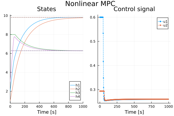
We test that the state converged to our reference and that the constraints were met.
using Test
@test sol(1000.0, idxs = [ssys.plant_nl.h1, ssys.plant_nl.h2, ssys.plant_nl.h3, ssys.plant_nl.h4]) ≈ xr atol = 0.1

U = reduce(hcat, sol(0:2:1000, idxs = [ssys.mpc_nl.u[1], ssys.mpc_nl.u[2]]).u)
@test all(maximum(U, dims = 2) .< 0.6 + 1e-2)
@test all(minimum(U, dims = 2) .> 0.0 - 1e-2)
Test PassedAs we can see, the nonlinear MPC controller performs quite well and respects the state constraints: the level of tank 3 remains at its upper bound during the first part of the transient instead of exceeding it, since the controller predicts with the nonlinear model and receives the measured levels directly, and acados reports a successful solve at every sample.
Summary
We have seen how to define and simulate linear and nonlinear MPC controllers with constraints on the inputs and the state of a nonlinear MIMO process.