
Cart-pole MPC with a penalty on the control increments
Below, we design an MPC controller for the nonlinear pendulum-on-a-cart system. This is the introductory example of the DyadControlSystems documentation for MPC with generic cost and constraints, here with the component ACADOSMPC as the controller. An additional example is available in the tutorial
The dynamics of the cart-pole are given by the component CartPolePlant, which is available as MPCComponents.Examples.CartPolePlant. The state consists of the cart position p, the pendulum angle th, which is zero when the pendulum hangs down, the cart velocity v and the pendulum angular velocity w, and the input is the force F on the cart:
"""
Cart-pole: a cart of mass `mc` driven by the force `F`, carrying a pendulum of mass `mp` and length `l`.
The angle `theta` is zero when the pendulum hangs down. Translated from the DyadControlSystems
quadratic-MPC tutorial.
"""
component CartPolePlant
  "Force on the cart"
  F = RealInput() {^F}
  "Cart position"
  pos = RealOutput() {^pos}
  "Pendulum angle"
  theta = RealOutput() {^theta}
  "Cart velocity"
  vel = RealOutput() {^vel}
  "Pendulum angular velocity"
  omega = RealOutput() {^omega}
  parameter mc::Real = 1.0
  parameter mp::Real = 0.2
  parameter l::Real = 0.5
  parameter g::Real = 9.81
  parameter p0::Real = 0.0
  parameter th0::Real = 0.0
  parameter v0::Real = 0.0
  parameter w0::Real = 0.0
  variable p::Real
  variable th::Real
  variable v::Real
  variable w::Real
relations
  initial p = p0
  initial th = th0
  initial v = v0
  initial w = w0
  der(p) = v
  der(th) = w
  der(v) = (F + mp * l * sin(th) * w ^ 2 + mp * g * sin(th) * cos(th)) / (mc + mp * sin(th) ^ 2)
  der(w) = -(cos(th) * (F + mp * l * sin(th) * w ^ 2) + (mc + mp) * g * sin(th)) / (l * (mc + mp * sin(th) ^ 2))
  pos = p
  theta = th
  vel = v
  omega = w
metadata {
  "Dyad": {
    "icons": {"default": "dyad://MPCComponents/CartPolePlant.svg"},
    "doc": {"behavior": false}
  },
  "_links": {
    "F": {
      "Dyad": {"placement": {"diagram": {"x1": -100, "x2": 0, "y1": 450, "y2": 550}}}
    },
    "pos": {
      "Dyad": {"placement": {"diagram": {"x1": 1000, "x2": 1100, "y1": 100, "y2": 200}}}
    },
    "theta": {
      "Dyad": {"placement": {"diagram": {"x1": 1000, "x2": 1100, "y1": 330, "y2": 430}}}
    },
    "vel": {
      "Dyad": {"placement": {"diagram": {"x1": 1000, "x2": 1100, "y1": 610, "y2": 710}}}
    },
    "omega": {
      "Dyad": {"placement": {"diagram": {"x1": 1000, "x2": 1100, "y1": 830, "y2": 930}}}
    }
  }
}
end
The state dimension is 4 and the system has a single input. The sample time is Ts = 0.1, the MPC optimization horizon is Np = 10, all four state variables start at 1 (the parameters p0, th0, v0 and w0 of the plant), and the reference is the origin. A controller that regulates to the origin rather than tracking a reference is obtained with reference_tracking = false, which removes the reference input r:
periodicclock = DiscreteComponents.PeriodicClock(dt = 0.1)
plant = CartPolePlant(p0 = 1.0, th0 = 1.0, v0 = 1.0, w0 = 1.0)
mpc = MPCComponents.ACADOSMPC(dynamics = plant,
                              inputs = ["F"],
                              state_variables = ["p", "th", "v", "w"],
                              Ts = 0.1,
                              Np = 10,
                              reference_tracking = false,
                              ...)
The prediction model is the plant component itself, dynamics = plant, and the entire state is available for measurement: four Sampler components sample the state of the plant once every Ts. acados integrates the continuous-time prediction model over each shooting interval, here with an implicit Runge-Kutta integrator with 3 stages:
integrator = MPCComponents.ACADOSIntegrator.IRK(),
integrator_stages = 3,
Objective
The objective consists of a running cost ACADOSMPC penalizes the controlled outputs named by outputs, here the full state, and the difference cost is enabled by penalize_increments = true:
outputs = ["p", "th", "v", "w"],
Q1 = diagonal([1.0, 1.0, 1.0, 1.0]),
Q2 = diagonal([0.1]),
penalize_increments = true,
Q3 = diagonal([0.1]),
The weights are matrices, and diagonal constructs a diagonal matrix from a vector. The terminal weight Qf defaults to Q1. ACADOSMPC can instead use the infinite-horizon LQR cost of the model linearized at an operating point as terminal cost (terminal_lqr_cost = true); this example uses the default.
The solver requires an initial guess of the trajectories. At the first sample, ACADOSMPC initializes the predicted state trajectory with the measured state (or with x_guess when it is given) and the control trajectory with u_guess, which is zero when it is not given, as here. At every subsequent sample, the solver starts from the solution of the previous sample.
Constraints
The control signal is constrained to umin and umax bound the control input, while constrained names the constrained signals of the model with their bounds in constrained_min and constrained_max:
umin = [-3.0],
umax = [3.0],
constrained = ["w"],
constrained_min = [-4.0],
constrained_max = [4.0],
The control bounds are hard. The state bounds are soft by default (state_bounds_soft = true), with a quadratic penalty on the constraint violation weighted by soft_weight; state_bounds_soft = false makes them hard.
Observer, solver and problem
The four samplers feed the state of the plant directly to the controller, i.e., the controller uses state feedback. The optimization problems are solved by acados using sequential quadratic programming, where each quadratic subproblem is solved by HPIPM. The closed-loop model below connects the plant, the samplers, the controller and a zero-order hold that holds the force between samples; the variables pos, theta, omega, u1 and flag make the signals of interest available for plotting, flag being the acados status of each solve (0 indicates success).
"""
The cart-pole example of the DyadControlSystems generic-MPC documentation ("Getting started"): all four
state variables start at 1 and are regulated to the origin with `Q1 = I`, `Q2 = 0.1`, a penalty
`Q3 = 0.1` on the force increments, the force bounded to ±3 and the pendulum angular velocity to ±4
(soft here, where the tutorial's stage constraint is hard). The tutorial's LQR-based terminal cost is
replaced by the default `Qf = Q1`.
"""
example component CartPoleIncrementMPCExample
  periodicclock = DiscreteComponents.PeriodicClock(dt = 0.1) {^periodicclock}
  plant = CartPolePlant(p0 = 1.0, th0 = 1.0, v0 = 1.0, w0 = 1.0) {^plant}
  "Samplers of the four state variables"
  s = [DiscreteComponents.Sampler() for i in 1:4] {^s}
  zoh = DiscreteComponents.ZeroOrderHold() {^zoh}
  mpc = MPCComponents.ACADOSMPC(dynamics = plant, inputs = ["F"], state_variables = ["p", "th", "v", "w"], outputs = ["p", "th", "v", "w"], Ts = 0.1, Np = 10, Q1 = diagonal([1.0, 1.0, 1.0, 1.0]), Q2 = diagonal([0.1]), penalize_increments = true, Q3 = diagonal([0.1]), umin = [-3.0], umax = [3.0], constrained = ["w"], constrained_min = [-4.0], constrained_max = [4.0], reference_tracking = false, integrator = MPCComponents.ACADOSIntegrator.IRK(), integrator_stages = 3) {^mpc}
  "Cart position"
  variable pos::Real
  "Pendulum angle"
  variable theta::Real
  "Pendulum angular velocity"
  variable omega::Real
  "Force"
  variable u1::Real
  "acados status"
  variable flag::Real
relations
  pos = plant.pos
  theta = plant.theta
  omega = plant.omega
  u1 = mpc.u[1]
  flag = mpc.exitflag
  connect(plant.pos, s[1].u)
  connect(plant.theta, s[2].u)
  connect(plant.vel, s[3].u)
  connect(plant.omega, s[4].u)
  connect(s[1].y, mpc.x[1], periodicclock.y)
  for i in 2:4
    connect(s[i].y, mpc.x[i])
  end
  connect(mpc.u[1], zoh.u) {^id6}
  connect(zoh.y, plant.F) {^id7}
metadata {
  "_links": {
    "periodicclock": {},
    "plant": {},
    "s": {},
    "zoh": {},
    "mpc": {},
    "id6": {},
    "id7": {}
  }
}
end
We instantiate the model in Julia and compile it. Models that contain clocked (discrete-time) components, such as the controller, are compiled with the additional pass SynchToolkit.compile_lustre, which compiles the discrete-time partitions of the model.
@named model = CartPoleIncrementMPCExample()
ssys = mtkcompile(model; additional_passes = [SynchToolkit.compile_lustre])
Run MPC controller
We simulate the closed-loop system over 100 sample intervals and plot the four state variables and the control signal, together with the bounds on the angular velocity and the force:
prob = ODEProblem(ssys, [], (0.0, 10.0))
sol = solve(prob)
plot(sol, idxs = [ssys.plant.p, ssys.plant.th, ssys.plant.v, ssys.plant.w, ssys.u1], layout = 5, lab = "",
     title = ["p" "th" "v" "w" "u"], xlabel = "Time [s]")
hline!([-4.0 4.0], sp = 4, l = (:black, :dash), lab = "")
hline!([-3.0 3.0], sp = 5, l = (:black, :dash), lab = "")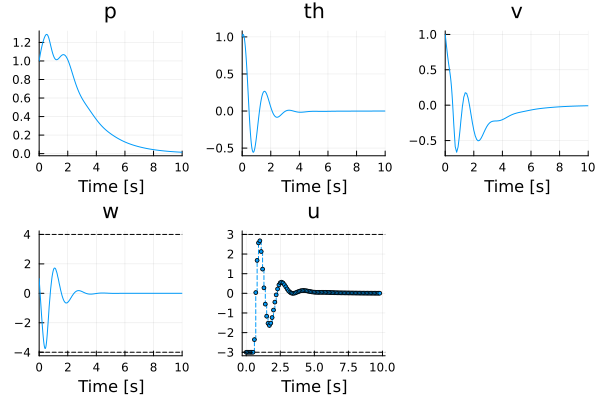
The controller regulates all four state variables to the origin, i.e., the cart returns to the origin and the pendulum comes to rest in the downward position: the pendulum angle has settled after approximately 3 s and the cart position after approximately 8 s. The force is at its lower bound during the first samples, and the angular velocity remains within its bounds throughout.