
Download as a Dyad projectDisturbanceRejection.zipOpen in Dyad Studio
Disturbance modeling and rejection with MPC controllers
This example will demonstrate how you can add disturbance models to a plant model and achieve effective disturbance rejection using an MPC controller. For simplicity, we will consider a simple first-order system
where a load disturbance
We will begin by setting up the MPC problem and solve it without any disturbance model. For details regarding the setup of an MPC problem, see the documentation of LinearMPCController.
We start by defining the process model, the transfer function
"First-order plant G(s) = k / (T s + 1) with a load disturbance added at the input."
component FirstOrderLoadPlant
  "Control input"
  u = RealInput() {^u}
  "Load disturbance acting at the input"
  d = RealInput() {^d}
  "Output"
  y = RealOutput() {^y}
  parameter T::Real = 10.0
  parameter k::Real = 1.0
  variable x::Real
relations
  initial x = 0.0
  der(x) = (k * (u + d) - x) / T
  y = x
metadata {
  "Dyad": {
    "icons": {"default": "dyad://MPCComponents/FirstOrderLoadPlant.svg"},
    "doc": {"behavior": false}
  },
  "_links": {
    "u": {
      "Dyad": {"placement": {"diagram": {"x1": -100, "x2": 0, "y1": 650, "y2": 750}}}
    },
    "d": {
      "Dyad": {"placement": {"diagram": {"x1": -100, "x2": 0, "y1": 220, "y2": 320}}}
    },
    "y": {
      "Dyad": {"placement": {"diagram": {"x1": 1000, "x2": 1100, "y1": 450, "y2": 550}}}
    }
  }
}
end
The controller is a LinearMPCController, whose prediction model is given by the matrices A, B and C of the same system. With continuous = true, the controller discretizes the model using zero-order hold with the sample time Ts, which is also the period of the clock that triggers the controller. The prediction horizon is Np = 10, the control signal is limited to Q1 = 100 and the control signal by Q2 = 0.01. The state is estimated by a steady-state Kalman filter with the process-noise covariance R1 and the measurement-noise covariance R2. The quadratic programs are solved by the DAQP solver, for which LinearMPC.jl generates C code.
mpc_none = MPCComponents.LinearMPCController(A = [[-0.1]], B = [[0.1]], C = [[1.0]], continuous = true, Ts = 1.0, Np = 10, Q1 = [100.0], Q2 = [0.01], umin = [-1.1], umax = [1.1], R1 = [0.001], R2 = [1.0])The initial state of the plant and of the estimate is zero, and so is the reference, provided by a Constant source. The load disturbance is a Step source connected to the input d of the plant.
The closed-loop model below contains two control loops that are identical except for the controller: mpc_none is the controller above, without a disturbance model, and mpc_of is a controller with a disturbance model, which we will discuss below. Both plants are subject to the same load disturbance.
"""
Load-disturbance rejection with `LinearMPCController` on the first-order plant 1/(10s+1): a unit step
load disturbance enters at the input at t = 10. Without a disturbance model the controller leaves a
steady-state offset; with the offset-free observer the output returns to the reference and the control
settles at -1. The observer is the tutorial's: a constant load disturbance on the input
(`offset_free = InputDisturbance`) estimated by a Kalman filter on the augmented model with the
tutorial's covariances `R1 = diag(0.001, 0.1)`, whose disturbance entry sets the estimation speed (the
tutorial lowers it from 1 to 0.1 to reduce the sensitivity peak). Translated from the DyadControlSystems
disturbance-rejection tutorial.
"""
example component DisturbanceRejectionMPCExample
  periodicclock = DiscreteComponents.PeriodicClock(dt = 1.0) {^periodicclock}
  plant_none = FirstOrderLoadPlant() {^plant_none}
  plant_of = FirstOrderLoadPlant() {^plant_of}
  dist = BlockComponents.Sources.Step(height = 1.0, start_time = 10.0) {^dist}
  ref = BlockComponents.Sources.Constant(k = 0.0) {^ref}
  sr = DiscreteComponents.Sampler() {^sr}
  s_none = DiscreteComponents.Sampler() {^s_none}
  s_of = DiscreteComponents.Sampler() {^s_of}
  zoh_none = DiscreteComponents.ZeroOrderHold() {^zoh_none}
  zoh_of = DiscreteComponents.ZeroOrderHold() {^zoh_of}
  mpc_none = MPCComponents.LinearMPCController(A = [[-0.1]], B = [[0.1]], C = [[1.0]], continuous = true, Ts = 1.0, Np = 10, Q1 = [100.0], Q2 = [0.01], umin = [-1.1], umax = [1.1], R1 = [0.001], R2 = [1.0]) {^mpc_none}
  mpc_of = MPCComponents.LinearMPCController(A = [[-0.1]], B = [[0.1]], C = [[1.0]], continuous = true, Ts = 1.0, Np = 10, Q1 = [100.0], Q2 = [0.01], umin = [-1.1], umax = [1.1], R1 = [0.001, R1_dist], R2 = [1.0], offset_free = MPCComponents.OffsetFreeMethod.InputDisturbance()) {^mpc_of}
  "Output without a disturbance model"
  variable y_none::Real
  "Output with the offset-free observer"
  variable y_of::Real
  "Process-noise covariance of the disturbance state in the observer of `mpc_of`"
  structural parameter R1_dist::Real = 0.1
  "Control with the offset-free observer"
  variable u_of::Real
relations
  y_none = plant_none.y
  y_of = plant_of.y
  u_of = mpc_of.u[1]
  connect(ref.y, sr.u)
  connect(dist.y, plant_none.d, plant_of.d)
  connect(plant_none.y, s_none.u)
  connect(s_none.y, mpc_none.y[1], periodicclock.y)
  connect(sr.y, mpc_none.r[1], mpc_of.r[1])
  connect(mpc_none.u[1], zoh_none.u)
  connect(zoh_none.y, plant_none.u)
  connect(plant_of.y, s_of.u)
  connect(s_of.y, mpc_of.y[1])
  connect(mpc_of.u[1], zoh_of.u)
  connect(zoh_of.y, plant_of.u)
metadata {
  "Dyad": {"doc": {"behavior": false}},
  "_links": {
    "periodicclock": {},
    "plant_none": {},
    "plant_of": {},
    "dist": {},
    "ref": {},
    "sr": {},
    "s_none": {},
    "s_of": {},
    "zoh_none": {},
    "zoh_of": {},
    "mpc_none": {},
    "mpc_of": {}
  }
}
end
We instantiate and compile the model, and simulate it for 100 sample intervals. Models that contain clocked (discrete-time) components, such as the controllers, are compiled with the additional pass SynchToolkit.compile_lustre. We first plot the output and the control signal of the loop without a disturbance model:
@named model = DisturbanceRejectionMPCExample()
ssys = mtkcompile(model; additional_passes = [SynchToolkit.compile_lustre])
prob = ODEProblem(ssys, [], (0.0, 100.0))
sol = solve(prob)
plot(sol, idxs = [ssys.y_none, ssys.mpc_none.u[1]], layout = (2, 1), lab = ["y" "u"], xlabel = "Time")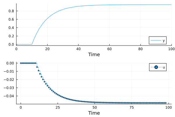
As we can see, the controller appears to do very little to suppress the disturbance. The problem is that the observer does not have a model for such a disturbance, and its estimate of the state will thus be severely biased.
The next step is to add a disturbance model to the plant model. Since the disturbance is of low-frequency character (indeed, its transfer function is offset_free = MPCComponents.OffsetFreeMethod.InputDisturbance(). The controller then augments its model with one integrating disturbance state per input and estimates the disturbance together with the state.
There is no point trying to penalize the disturbance state in the MPC optimization, since it is not controllable. Q1 of LinearMPCController penalizes the controlled outputs
The controller uses the disturbance estimate in its prediction, which gives offset-free control under constant disturbances.
The Kalman filter of the augmented model takes a process-noise covariance R1 with one entry for the state of the plant and one for the disturbance state. The entry that corresponds to the disturbance state determines how fast the Kalman filter integrates the disturbance. We choose a large value, implying fast integration:
mpc_of = MPCComponents.LinearMPCController(A = [[-0.1]], B = [[0.1]], C = [[1.0]], continuous = true, Ts = 1.0, Np = 10, Q1 = [100.0], Q2 = [0.01], umin = [-1.1], umax = [1.1], R1 = [0.001, R1_dist], R2 = [1.0], offset_free = MPCComponents.OffsetFreeMethod.InputDisturbance())The disturbance entry is the structural parameter R1_dist of the example model, which defaults to a smaller value that we will come back to below. Here, we replace it with the large value when we instantiate the model:
@named model_fast = DisturbanceRejectionMPCExample(R1_dist = 1.0)
ssys_fast = mtkcompile(model_fast; additional_passes = [SynchToolkit.compile_lustre])
prob_fast = ODEProblem(ssys_fast, [], (0.0, 100.0))
sol_fast = solve(prob_fast)
plot(sol_fast, idxs = [ssys_fast.y_of, ssys_fast.u_of], layout = (2, 1), lab = ["y" "u"], xlabel = "Time")
ylims!((-0.05, 0.3), sp = 1)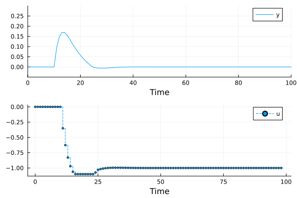
This time around we see that the controller indeed rejects the disturbance, and after a few samples at its lower bound the control signal settles on -1, which is exactly what is required to counteract the load disturbance of +1.
Before we feel confident about deploying the MPC controller, we would investigate its closed-loop properties. The DyadControlSystems version of this tutorial does so by computing the sensitivity functions of the linear controller that is equivalent to the unconstrained MPC controller, and finds a rather high peak in the sensitivity function. This is an indication that we perhaps added too much "integral action" by a too fast observer pole related to the disturbance state. Such a closed-loop analysis is not covered here; instead, we investigate how a slightly more conservative design fares. The controller mpc_of of the example model is this design, with the disturbance entry of R1 lowered to the default R1_dist = 0.1, and we plot its response from the solution sol computed above:
plot(sol, idxs = [ssys.y_of, ssys.u_of], layout = (2, 1), lab = ["y" "u"], xlabel = "Time")
ylims!((-0.05, 0.3), sp = 1)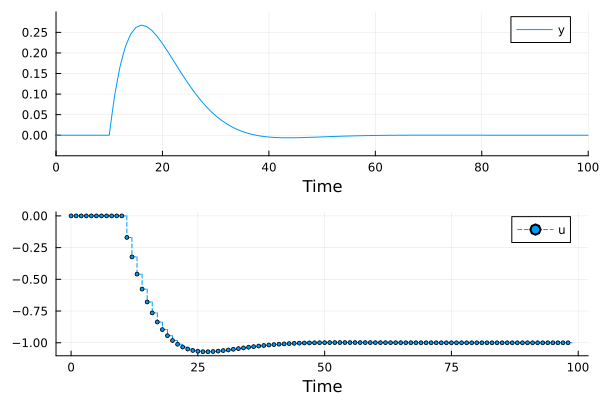
We see that we now have a larger disturbance response than before: the peak of the output increases from about 0.17 to about 0.27, and the output returns to the reference more slowly, while the control signal no longer reaches its bound. The purpose of this design, according to the closed-loop analysis in the DyadControlSystems version of this tutorial, is a lower peak of the sensitivity and complementary sensitivity functions, i.e., a more robust design, and a reduced amplification of measurement noise (
using Test
@test sol(100.0, idxs = ssys.y_of) ≈ 0 atol = 1e-5
@test sol(100.0, idxs = ssys.u_of) ≈ -1 atol = 1e-5
Test Passed