
MPC for autonomous lane changes
In this example, we will develop a lane-changing controller using Model-Predictive Control (MPC). We will use a dynamical model of the car that is sometimes referred to as the kinematic bicycle model, given by the following equations
Where
After having loaded the necessary packages
using MPCComponents
using ModelingToolkit
using SynchToolkit
using OrdinaryDiffEqDefault
import BlockComponents
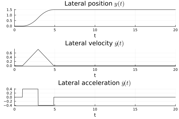
using PlotsPlots.GRBackend()we generate a reference trajectory for the lateral position y with bounded velocities and accelerations. For this, we make use of the component BlockComponents.Sources.KinematicPTP, which generates a point-to-point trajectory from q0 to q1 with the velocity bounded by qd_max and the acceleration bounded by qdd_max, starting at startTime. The reference moves the car one lane over, 1.5 m to the left, with the lateral velocity bounded by 1.5 m/s and the lateral acceleration bounded by 0.4 m/s². The DyadControlSystems version of this example instead filters a square wave that alternates between the two lanes, so that the car changes lanes repeatedly, while this example performs a single lane change:
yref = BlockComponents.Sources.KinematicPTP(q0 = [0.0], q1 = [1.5], qd_max = [1.5], qdd_max = [0.4], startTime = 1.0)The component outputs the position q, the velocity qd and the acceleration qdd of the trajectory. We simulate it on its own to show the profile. Over this distance, the acceleration bound determines the profile, and the lateral velocity remains below its bound:
@named yref = BlockComponents.Sources.KinematicPTP(q0 = [0.0], q1 = [1.5], qd_max = [1.5], qdd_max = [0.4], startTime = 1.0)
ssys_ref = mtkcompile(yref)
prob_ref = ODEProblem(ssys_ref, [], (0.0, 20.0))
sol_ref = solve(prob_ref)
plot(
    sol_ref,
    idxs   = [ssys_ref.q[1], ssys_ref.qd[1], ssys_ref.qdd[1]],
    c      = :black,
    title  = ["Lateral position \$y(t)\$" "Lateral velocity \$\\dot{y}(t)\$" "Lateral acceleration \$\\ddot y(t)\$"],
    ylabel = "",
    lab    = "",
    layout = (3, 1),
)
We now define the dynamics and specify that we can measure all three state variables, MPCComponents.Examples.LaneChangeCarPlant, whose definition we reproduce below. The heading deg, so that the heading and its derivative are expressed in the same unit.
"""
Kinematic bicycle model of a car for lane changes: lateral position `y`, speed `v` and heading `psi`
(degrees), driven by the acceleration `a` and the steering angle `delta` (degrees). Unlike the
DyadControlSystems lane-change tutorial, which treats `v tan(delta) / L` directly as a heading rate in
degrees per second, the heading rate here is converted consistently to degrees.
"""
component LaneChangeCarPlant
  "Acceleration"
  a = RealInput() {^a}
  "Steering angle (degrees)"
  delta = RealInput() {^delta}
  "Lateral position"
  y_out = RealOutput() {^y_out}
  "Speed"
  v_out = RealOutput() {^v_out}
  "Heading (degrees)"
  psi_out = RealOutput() {^psi_out}
  "Distance between the axles"
  parameter L::Real = 2.9
  parameter y0::Real = 0.0
  parameter v0::Real = 8.333333333333334
  parameter psi0::Real = 0.0
  "Degrees per radian"
  final parameter deg::Real = 57.29577951308232
  variable y::Real
  variable v::Real
  variable psi::Real
relations
  initial y = y0
  initial v = v0
  initial psi = psi0
  der(y) = v * sin(psi / deg)
  der(v) = a
  der(psi) = deg * v / L * tan(delta / deg)
  y_out = y
  v_out = v
  psi_out = psi
metadata {
  "Dyad": {
    "icons": {"default": "dyad://MPCComponents/LaneChangeCarPlant.svg"},
    "doc": {"behavior": false}
  },
  "_links": {
    "a": {
      "Dyad": {"placement": {"diagram": {"x1": -100, "x2": 0, "y1": 240, "y2": 340}}}
    },
    "delta": {
      "Dyad": {"placement": {"diagram": {"x1": -100, "x2": 0, "y1": 680, "y2": 780}}}
    },
    "y_out": {
      "Dyad": {"placement": {"diagram": {"x1": 1000, "x2": 1100, "y1": 170, "y2": 270}}}
    },
    "v_out": {
      "Dyad": {"placement": {"diagram": {"x1": 1000, "x2": 1100, "y1": 450, "y2": 550}}}
    },
    "psi_out": {
      "Dyad": {"placement": {"diagram": {"x1": 1000, "x2": 1100, "y1": 750, "y2": 850}}}
    }
  }
}
end
The controller is the component ACADOSMPC, which uses the plant component itself as its prediction model, with the inputs a and delta and the state variables y, v and psi. All three state variables are also the controlled outputs:
mpc = MPCComponents.ACADOSMPC(dynamics = plant,
                              inputs = ["a", "delta"],
                              state_variables = ["y", "v", "psi"],
                              outputs = ["y", "v", "psi"],
                              ...)
The controller operates with a sample time of PeriodicClock that triggers it and its parameter Ts. The plant is simulated in continuous time by an ODE solver, while the MPC controller internally integrates the prediction model over each sample interval with an implicit Runge-Kutta integrator (IRK) with 3 stages in this example:
periodicclock = DiscreteComponents.PeriodicClock(dt = 0.1)
Ts = 0.1,
integrator = MPCComponents.ACADOSIntegrator.IRK(),
integrator_stages = 3,
Next up, we define an initial condition y0, v0 and psi0 of LaneChangeCarPlant, with the initial velocity 30 km/h. The reference for the velocity is 50 km/h, and the reference for the heading is zero:
vref = BlockComponents.Sources.Constant(k = 13.88888888888889)
psiref = BlockComponents.Sources.Constant(k = 0.0)
The controller receives the current value of the reference at every sample and holds it constant over the prediction horizon (reference_preview would instead provide a reference trajectory over the horizon). We will limit the velocity to 120km/h (and divide by 3.6 to get m/s), the acceleration to be within
umin = [-10.0, -25.0],
umax = [1.96, 25.0],
constrained = ["y", "v", "psi"],
constrained_min = [-1.53, 0.0, -6.0],
constrained_max = [1.53, 33.333333333333336, 6.0],
The control bounds are hard, while the state bounds are soft by default (state_bounds_soft), with a quadratic penalty on the constraint violation weighted by soft_weight. For improved numerics, ACADOSMPC accepts scaling vectors x_scale and u_scale that indicate the typical magnitudes of the state components and inputs. The controller in this example converges without scaling, and we therefore leave these parameters at their default values.
The cost function will be quadratic and we will penalize the deviation from the reference trajectory with Q1. We will also penalize the control inputs Q2 to avoid large accelerations and steering angles, and control input differences Q3 to avoid high jerk (high jerk causes neck discomfort):
Q1 = diagonal([1.0, 0.02, 0.01]),
Q2 = diagonal([0.01, 1e-5]),
penalize_increments = true,
Q3 = diagonal([1.0, 0.001]),
The weights are matrices, and diagonal constructs a diagonal matrix from a vector. With penalize_increments = true, the prediction model is augmented with the control signal as a state, and the control rate becomes the decision variable of the optimization problem.
To improve the stability properties of an MPC controller, a terminal constraint may enforce the final state to be equal to the reference state; ACADOSMPC provides such constraints through terminal_constrained, terminal_constrained_min and terminal_constrained_max. This example does not impose a terminal constraint, and the objective instead contains the terminal cost with the weight Qf, which defaults to Q1. The prediction horizon is
Np = 30,The solver requires an initial guess for the optimal solution. At the first sample, ACADOSMPC initializes the predicted trajectories with the measured state and the control u_guess, which is zero when it is not given. At every subsequent sample, the solver starts from the solution of the previous sample, shifted by one step.
The optimization problems are solved by acados using sequential quadratic programming (nlp_solver = SQP, the default), where each quadratic subproblem is solved by HPIPM, with the Gauss-Newton approximation of the Hessian of the least-squares objective. The samplers s provide the state of the plant to the controller directly, which indicates that we have perfect knowledge of the state.
We are now ready to construct the closed-loop model. The samplers sr sample the three references, and the zero-order holds zoh hold the controls between samples. The variables y, r, v, psi, a, delta and flag make the signals of interest available for plotting, flag being the acados status of each solve (0 indicates success).
"""
Autonomous lane change with `ACADOSMPC`, translated from the DyadControlSystems lane-change tutorial:
the car follows a smooth lateral reference (a point-to-point profile with bounded lateral velocity and
acceleration, in place of the tutorial's trajectory limiter) from one lane to the next while
accelerating from 30 to 50 km/h, with the tutorial's weights on the state, the controls and the control
increments and its bounds on the lateral position, speed, heading, acceleration and steering angle.
The reference is held constant over the horizon (no preview) and the tutorial's terminal equality
constraint is not imposed.
"""
example component LaneChangeMPCExample
  periodicclock = DiscreteComponents.PeriodicClock(dt = 0.1) {^periodicclock}
  plant = LaneChangeCarPlant() {^plant}
  "Samplers of the three state variables"
  s = [DiscreteComponents.Sampler() for i in 1:3] {^s}
  "Reference samplers"
  sr = [DiscreteComponents.Sampler() for i in 1:3] {^sr}
  "Holds of the acceleration and the steering angle"
  zoh = [DiscreteComponents.ZeroOrderHold() for i in 1:2] {^zoh}
  "Lateral reference: one lane over, with bounded lateral velocity and acceleration"
  yref = BlockComponents.Sources.KinematicPTP(q0 = [0.0], q1 = [1.5], qd_max = [1.5], qdd_max = [0.4], startTime = 1.0) {^yref}
  "Speed reference, 50 km/h"
  vref = BlockComponents.Sources.Constant(k = 13.88888888888889) {^vref}
  "Heading reference"
  psiref = BlockComponents.Sources.Constant(k = 0.0) {^psiref}
  mpc = MPCComponents.ACADOSMPC(dynamics = plant, inputs = ["a", "delta"], state_variables = ["y", "v", "psi"], outputs = ["y", "v", "psi"], Ts = 0.1, Np = 30, Q1 = diagonal([1.0, 0.02, 0.01]), Q2 = diagonal([0.01, 1e-5]), penalize_increments = true, Q3 = diagonal([1.0, 0.001]), umin = [-10.0, -25.0], umax = [1.96, 25.0], constrained = ["y", "v", "psi"], constrained_min = [-1.53, 0.0, -6.0], constrained_max = [1.53, 33.333333333333336, 6.0], integrator = MPCComponents.ACADOSIntegrator.IRK(), integrator_stages = 3) {^mpc}
  "Lateral position"
  variable y::Real
  "Lateral reference"
  variable r::Real
  "Speed"
  variable v::Real
  "Heading (degrees)"
  variable psi::Real
  "Acceleration"
  variable a::Real
  "Steering angle (degrees)"
  variable delta::Real
  "acados status"
  variable flag::Real
relations
  y = plant.y
  r = yref.q[1]
  v = plant.v
  psi = plant.psi
  a = mpc.u[1]
  delta = mpc.u[2]
  flag = mpc.exitflag
  connect(plant.y_out, s[1].u)
  connect(plant.v_out, s[2].u)
  connect(plant.psi_out, s[3].u)
  connect(yref.q[1], sr[1].u)
  connect(vref.y, sr[2].u)
  connect(psiref.y, sr[3].u)
  connect(s[1].y, mpc.x[1], periodicclock.y)
  for i in 2:3
    connect(s[i].y, mpc.x[i])
  end
  for i in 1:3
    connect(sr[i].y, mpc.r[i])
  end
  for i in 1:2
    connect(mpc.u[i], zoh[i].u)
  end
  connect(zoh[1].y, plant.a)
  connect(zoh[2].y, plant.delta)
metadata {
  "Dyad": {"doc": {"behavior": false}},
  "_links": {
    "periodicclock": {},
    "plant": {},
    "s": {},
    "sr": {},
    "zoh": {},
    "yref": {},
    "vref": {},
    "psiref": {},
    "mpc": {}
  }
}
end
We instantiate the model in Julia and compile it. Models that contain clocked (discrete-time) components, such as the controller, are compiled with the additional pass SynchToolkit.compile_lustre, which compiles the discrete-time partitions of the model.
@named model = LaneChangeMPCExample()
ssys = mtkcompile(model; additional_passes = [SynchToolkit.compile_lustre])
We simulate the closed-loop system for 20 seconds, i.e., 200 samples, and plot the result, with the references shown dashed:
prob = ODEProblem(ssys, [], (0.0, 20.0))
sol = solve(prob)
fx = plot(sol, idxs = [ssys.y, ssys.v, ssys.psi], layout = 3, lab = ["y" "v" "ψ"])
plot!(sol, idxs = [ssys.r], sp = 1, l = (:black, :dash), lab = "yᵣ")
hline!([sol.ps[ssys.vref.k]], sp = 2, l = (:black, :dash), lab = "vᵣ")
hline!([sol.ps[ssys.psiref.k]], sp = 3, l = (:black, :dash), lab = "ψᵣ")
plot(fx, plot(sol, idxs = [ssys.a, ssys.delta], layout = 2, lab = ["a" "δ"]))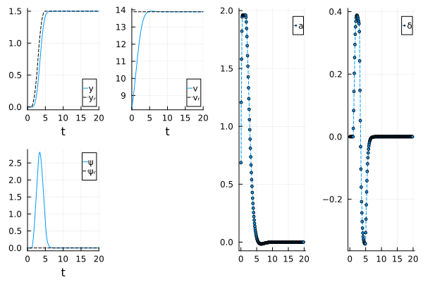
The lateral position follows the reference with a small delay, the largest deviation being 0.41 m during the lane change, and the car is in the new lane less than a second after the reference has arrived there. The velocity reaches 50 km/h after approximately 4 seconds, with the acceleration at its upper bound
Finally, we produce a little animation of the car changing lanes. To get the
let
    t = range(0, 20, length = 2001)
    v = sol(t, idxs = ssys.v).u
    ψ = sol(t, idxs = ssys.psi).u
    ẋ = v .* cosd.(ψ)
    x = [0; cumsum((ẋ[1:end-1] .+ ẋ[2:end]) ./ 2 .* step(t))] # trapezoidal integration
    y = sol(t, idxs = ssys.y).u
    anim = Plots.Animation()

    x_coords = [-1, 1, 1, -1, -1]
    y_coords = 0.2*[-1, -1, 1, 1, -1]
    car = Shape(x_coords, y_coords)

    for i in 1:20:length(t)
        fig = plot(x[1:i], y[1:i],
            ylabel  = "",
            legend  = false,
            lab     = "History",
            ylims = (-2.3, 2.3),
            xlims = (-1, x[end] + 1),
            size =  (1300, 120),
            framestyle = :none,
        )
        hline!([-0.75 0.75], c = :black, l = :dash, primary=false)
        hline!([-2.25 2.25], c = :black, primary=false)
        cari = Plots.rotate(car, deg2rad(ψ[i]))
        cari = Plots.translate(cari, x[i], y[i])
        plot!(cari)
        frame(anim, fig)
    end
    gif(anim, fps = 25)
end
This concludes the example.
using Test
tk = 0:0.1:20
E_y = sol(tk, idxs = ssys.y) .- sol(tk, idxs = ssys.r)
E_v = sol(tk, idxs = ssys.v) .- sol.ps[ssys.vref.k]
@test sum(abs, E_y)/length(tk) < 0.1
@test sum(abs, E_v[50:end])/length(tk) < 0.5
Test Passed