
Download as a Dyad projectLinearMPC.zipOpen in Dyad Studio
Linear MPC
The component LinearMPCController implements linear MPC with a quadratic cost function and linear constraints, built on LinearMPC.jl. The optimization problem is a quadratic program (QP), which is condensed once when the model is built and solved at every sample instant by the active-set solver DAQP, in C code generated for the specific controller. This page describes the formulation; the parameters are listed in the documentation of LinearMPCController. For an introduction to MPC, see Model-predictive control.
Prediction model
The prediction model is the discrete-time linear system
with state
From a plant model. With dynamics = plant, where plant is a subcomponent of the closed-loop model declared before the controller, the controller linearizes the plant model at an operating point and discretizes the result with a zero-order hold and the sample interval Ts. The signals of the plant are referred to by name:
| Parameter | Signals | Role in the model |
|---|---|---|
inputs | control inputs | columns of |
known_disturbance_inputs | measured disturbances | columns of |
outputs | controlled and measured outputs | rows of |
disturbance_inputs | unmeasured inputs | set to zero in the prediction |
state_variables | state variables | order of xhat |
The operating point is selected by linearization_point: the initial state of the plant (InitialState), the steady state for given inputs (SteadyState), or the steady state at which the outputs take given values (OutputTarget). The offsets state_variables is required for all parameters that refer to individual state variables, such as R1 and Ax.
From matrices. Alternatively, the matrices A, B, Bd, C, Dd and the offsets f_offset and h_offset are given directly, in discrete time, or in continuous time with continuous = true, in which case they are discretized with the sample interval Ts.
Cost function
The controller minimizes, over the prediction horizon of
where
Q1weights the tracking errors of the controlled outputs. Withreference_tracking = falsethe reference is zero and the controller has no reference input.Q2weights the control signal and is zero by default. A nonzeroQ2penalizes the deviation offrom zero; since a nonzero control signal is in general required to hold the output at a nonzero reference, a nonzero Q2causes a steady-state error. For the same reason, the controller warns when a nonzeroQ2is combined with reference tracking on a plant without integral action.Q3weights the control increments. The increments are zero in steady state, so this term causes no steady-state error. It is the recommended way of regularizing the control signal.Qfis the terminal weight and defaults toQ1. It approximates the cost of the remainder of the trajectory beyond the horizon. For regulation to the origin of the state (reference_tracking = false),terminal_lqr_cost = truereplaces it by the infinite-horizon LQR cost-to-go, obtained from the discrete-time algebraic Riccati equation. With this terminal cost, the controller coincides with the LQR controller as long as no constraint is active.
The cost function may in addition contain a cross term
Constraints
| Constraint | Parameters | Type |
|---|---|---|
umin, umax | hard | |
dumin, dumax | hard, over the control horizon | |
ymin, ymax | soft by default | |
Ax, Au, Ar, Ad, Aup, Ap, lb, ub | hard by default |
A soft constraint may be violated, and the violation is penalized in the cost function with the weight soft_weight. Bounds on outputs and state variables should in general be soft: a disturbance or a model error may move the system to a state from which a hard output constraint cannot be satisfied, and the QP then has no solution. Bounds on the control signal are hard, since they describe physical limits of the actuators.
The output bounds and the general constraints are enforced at the prediction steps output_bounds_ks and constraint_ks, which default to binary_controls are restricted to the values umin and umax, which turns the QP into a mixed-integer QP (see MPC with binary or integer variables (MINLP)).
Horizons
The prediction horizon Np determines how far ahead the controller predicts. It should generally cover the time the closed-loop system requires to settle, or at least the dominant time constants of the plant. The control horizon Nc (default Np) is the number of steps over which the control signal is free; after it, the control signal is held constant. move_block keeps the control signal constant over blocks of steps of given lengths. Both reduce the number of decision variables, and thereby the computation time, at the expense of performance.
Observer
The state is estimated by a stationary Kalman filter, with the process-noise covariance R1 and the measurement-noise covariance R2:
The ratio of R1 to R2 determines how much the filter relies on the measurements relative to the model. The estimate is available as the output xhat.
A constant disturbance or a constant model error causes a steady-state error unless the model contains integral action. The parameter offset_free augments the model with constant disturbance states, which are estimated by the observer and included in the prediction: InputDisturbance adds a disturbance at every control input, OutputDisturbance a bias at every output, and StateDisturbance and Velocity are fixed-gain alternatives. Alternatively, a disturbance model is included in the Dyad plant model and its input is listed in disturbance_inputs. See Disturbance modeling and rejection with MPC controllers.
The observer and the optimizer are also available as the separate components LinearMPCObserver and LinearMPCOptimizer, e.g., to use the optimizer with a different state estimate.
Preview
With reference_preview, disturbance_preview or parameter_preview, the inputs r, d and p contain the values of the signal at every step of the prediction horizon instead of only the current value. The vector is ordered column-major: r[(j-1)*ny + i] is the reference for output i at prediction step j. A DelayLine assembles such a vector from a signal that is known in advance.
Solver
The QP is solved by DAQP. The output exitflag is 1 when the solution is optimal, 2 when it is optimal with active soft constraints, and negative when the solver fails. The solver runs in C code that LinearMPC.jl generates for the controller, which is also used when the model is exported with CCodeExport. All parameters of the controller are structural, since the QP is condensed when the model is built.
Example: reference tracking of a double integrator
The plant is a unit mass driven by a force
"""
Double integrator: a unit mass on a frictionless surface, driven by the force `u`. The state
consists of the position `x` and the velocity `v`, both of which are available as outputs.
"""
component DoubleIntegratorPlant
  "Force"
  u = RealInput() {^u}
  "Position"
  position = RealOutput() {^position}
  "Velocity"
  velocity = RealOutput() {^velocity}
  "Mass"
  parameter m::Real = 1.0
  "Initial position"
  parameter x0::Real = 0.0
  "Initial velocity"
  parameter v0::Real = 0.0
  "Position"
  variable x::Real(initial = x0)
  "Velocity"
  variable v::Real(initial = v0)
relations
  der(x) = v
  m * der(v) = u
  position = x
  velocity = v
metadata {
  "Dyad": {
    "icons": {"default": "dyad://MPCComponents/DoubleIntegratorExamplePlant.svg"},
    "doc": {"behavior": false}
  },
  "_links": {
    "u": {
      "Dyad": {"placement": {"diagram": {"x1": -100, "x2": 0, "y1": 450, "y2": 550}}}
    },
    "position": {
      "Dyad": {"placement": {"diagram": {"x1": 1000, "x2": 1100, "y1": 250, "y2": 350}}}
    },
    "velocity": {
      "Dyad": {"placement": {"diagram": {"x1": 1000, "x2": 1100, "y1": 650, "y2": 750}}}
    }
  }
}
end
The controller tracks a step in the position reference. Only the position is measured, and the velocity is estimated by the Kalman filter. The prediction model is obtained by linearizing the plant (dynamics = plant), and state_variables fixes the order of the state to
the sample interval
Ts = 0.1and the prediction horizonNp = 30, i.e., 3 s,the weight
Q1 = [1.0]on the tracking error of the position and the weightQ3 = [0.1]on the force increments;Q2is zero by default,the force bound
uminandumax,the velocity bound
Ax = [[0.0, 1.0]],lb = [-0.5]andub = [0.5],the covariances
R1andR2of the Kalman filter.
"""
Reference tracking with `LinearMPCController` on the double integrator `DoubleIntegratorPlant`. Only
the position is measured; the velocity is estimated by the Kalman filter of the controller. The
prediction model is obtained by linearizing the plant (`dynamics = plant`). The cost penalizes the
tracking error of the position and the increments of the force, the force is limited to
``|u| \\le 1`` and the velocity to ``|v| \\le 0.5`` through a general linear constraint on the state.
The position reference steps from 0 to 1 at t = 1.
"""
example component LinearMPCIntroExample
  periodicclock = DiscreteComponents.PeriodicClock(dt = 0.1) {^periodicclock}
  plant = DoubleIntegratorPlant() {^plant}
  ref = BlockComponents.Sources.Step(height = 1.0, start_time = 1.0) {^ref}
  sy = DiscreteComponents.Sampler() {^sy}
  sr = DiscreteComponents.Sampler() {^sr}
  zoh = DiscreteComponents.ZeroOrderHold() {^zoh}
  mpc = MPCComponents.LinearMPCController(dynamics = plant, inputs = ["u"], outputs = ["position"], state_variables = ["x", "v"], Ts = 0.1, Np = 30, Q1 = [1.0], Q3 = [0.1], umin = [-1.0], umax = [1.0], Ax = [[0.0, 1.0]], lb = [-0.5], ub = [0.5], R1 = [1e-4, 1e-2], R2 = [1e-4]) {^mpc}
  "Position"
  variable position::Real
  "Velocity"
  variable velocity::Real
  "Force"
  variable force::Real
  "Velocity estimated by the controller"
  variable velocity_estimate::Real
  "Exit flag of the QP solver"
  variable flag::Real
relations
  position = plant.position
  velocity = plant.velocity
  force = zoh.y
  velocity_estimate = mpc.xhat[2]
  flag = mpc.exitflag
  connect(plant.position, sy.u)
  connect(sy.y, mpc.y[1], periodicclock.y)
  connect(ref.y, sr.u)
  connect(sr.y, mpc.r[1])
  connect(mpc.u[1], zoh.u)
  connect(zoh.y, plant.u)
metadata {
  "Dyad": {"doc": {"behavior": false}},
  "_links": {
    "periodicclock": {},
    "plant": {},
    "ref": {},
    "sy": {},
    "sr": {},
    "zoh": {},
    "mpc": {}
  }
}
end
The PeriodicClock determines the sample instants, the samplers sy and sr sample the measured position and the reference, and the zero-order hold zoh holds the force between the sample instants.
@named model = LinearMPCIntroExample()
ssys = mtkcompile(model; additional_passes = [SynchToolkit.compile_lustre])
prob = ODEProblem(ssys, [], (0.0, 10.0))
sol = solve(prob)
plot(sol, idxs = [ssys.position, ssys.ref.y, ssys.velocity, ssys.velocity_estimate, ssys.force],
     layout = (3, 1), sp = [1 1 2 2 3], lab = ["position" "reference" "velocity" "velocity estimate" "force"],
     xlabel = "Time [s]", size = (700, 600))
hline!([0.5], sp = 2, l = (:black, :dash), lab = "")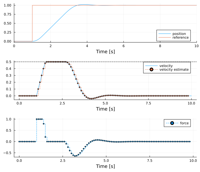
The force is at its upper bound until the velocity approaches its bound. The controller then holds the velocity at 0.5 and decelerates in time to reach the reference with a small overshoot. Since the controller predicts the step only from the moment it occurs, it does not act before reference_preview, the controller would start to move in advance. The velocity estimate of the Kalman filter is close to the actual velocity. DAQP returns the exit flag 1 at every sample instant.
using Test
@test all(==(1), sol[ssys.flag])
@test sol(10.0, idxs = ssys.position) ≈ 1 atol = 1e-4
@test maximum(abs, sol[ssys.velocity]) <= 0.5 + 1e-6
@test maximum(abs, sol[ssys.force]) <= 1 + 1e-9
Test Passed