
Nonlinear MPC
The component ACADOSMPC implements nonlinear MPC with the optimal-control solver acados. The prediction model is a nonlinear, continuous-time model, typically the Dyad model of the plant itself or a simplified version thereof. At every sample instant, the controller solves a nonlinear optimal-control problem by sequential quadratic programming (SQP), starting from the solution of the previous sample instant. This page describes the formulation; the parameters are listed in the documentation of ACADOSMPC. For an introduction to MPC, see Model-predictive control, and for the linear counterpart, see Linear MPC.
Prediction model
The prediction model is the continuous-time system
with state
A Dyad plant model. With
dynamics = plant, whereplantis a subcomponent of the closed-loop model, the controller uses the equations of the plant. The control inputs are listed ininputs, andstate_variablesnames the state variables in the order of the controller inputx. Inputs listed indisturbance_inputsare set to zero in the prediction. The parameters of the plant are replaced by their values, except those listed intunable_parameters, which become online parameters that can be changed without rebuilding the controller.A
ContinuousDynamicsobject, created bycontinuous_dynamicsfrom symbolic expressions or from a Julia function.A semi-explicit DAE of index 1, which requires the implicit integrator (
integrator = IRK).A discrete-time model
integrator = Discrete.
The prediction model must not contain events or explicit dependence on time; time-varying quantities enter as online parameters.
Discretization
acados discretizes the problem by multiple shooting: the horizon is divided into integrator = ERK, by default the classical fourth-order method) or implicit Runge-Kutta (integrator = IRK, Gauss-Legendre or Radau IIA collocation) for stiff models and DAEs. integrator_stages and integrator_steps select the number of stages and the number of integration steps per shooting interval.
An accurate integration is in general less important than a short sample interval: the prediction model is not exact, the feedback corrects the integration errors at the next sample instant, and a short sample interval improves the rejection of disturbances.
With time_steps, the intervals have individual lengths. The first interval always has the length geometric_time_steps and linear_time_steps construct such grids.
Cost function
The controller minimizes
where outputs, or nonlinear functions diagonal([1.0, 10.0]) constructs a diagonal matrix), and by default reference_tracking = false, the reference is zero and the controller has no reference input.
The increment penalty
Q3requirespenalize_increments = true, which augments the model with the control signal as an additional state variable and makes the rate of change of the control signal the decision variable.Q1andQ2may then be singular.With increments,
euandEuadd the direct economic input cost(Eu*p + eu)'uon both backends, including whenQ2 = 0. An absolute-input penalty throughQ2is optional. The first increment uses the previously applied command; subsequent increments use the preceding predicted command.Soft nonlinear stage and terminal constraints and nonlinear least-squares outputs can be combined with increments on both backends. Continuous-time prediction uses a ramp from the preceding command to the returned endpoint command; discrete-time prediction applies the endpoint command for the entire interval. Stage constraints use the boundary state and endpoint command. Terminal constraints use the terminal plant state. Convex-over-nonlinear constraints require the Julia backend.
terminal_lqr_cost = truereplaces the terminal term by the infinite-horizon LQR cost-to-go of the model linearized atoperating_point, which allows a short horizon to approximate the infinite-horizon controller near this point.The weights are tunable parameters: they can be changed after the model is compiled, without rebuilding the solver.
The least-squares terms use a Gauss–Newton Hessian, optionally regularized by levenberg_marquardt. The economic term contributes its exact gradient. Soft constraints add quadratic penalties on their lower and upper slacks at each applicable stage, including the terminal boundary, with coefficient soft_weight/2.
Constraints
| Constraint | Parameters | Type |
|---|---|---|
umin, umax | hard | |
dumin, dumax | hard | |
xmin, xmax, or constrained with constrained_min, constrained_max for named signals | soft by default | |
Ax, Au, lb, ub | hard | |
terminal_constrained, or AxN, lbN, ubN | hard unless terminal_constraints_soft | |
nl_constrained, nl_terminal_constrained | hard unless nl_constraints_soft |
Soft constraints are penalized quadratically with the weight soft_weight. As for linear MPC, state constraints should in general be soft, so that the problem remains feasible when a disturbance moves the system outside the constraints. A constraint nl_convex_inner and nl_convex_outer, which allows acados to include the curvature of
Scaling
When the state variables have very different magnitudes, x_scale and u_scale specify their typical magnitudes. The optimization is then performed in the scaled variables
Solver
With nlp_solver = SQP (the default), the SQP iterations continue until the tolerance tol or the iteration limit max_iter is reached. With SQP_RTI (real-time iteration), a single SQP iteration is performed at every sample instant, starting from the shifted solution of the previous sample instant. This reduces and bounds the computation time, and the solution converges over the following sample instants while the system moves. The quadratic subproblems are solved by HPIPM, after partial condensing (the default, qp_cond_N stages) or full condensing, or by DAQP after full condensing.
The four NLP stopping tests can use independent thresholds. nlp_tol_stat, nlp_tol_eq, nlp_tol_ineq and nlp_tol_comp correspond to stationarity, dynamics equality defects, inequality violations and complementarity. Each is a structural parameter: a positive value sets its threshold, while zero follows the tunable tol. Changing tol leaves positive overrides unchanged. Positive overrides require nlp_solver = SQP, since SQP_RTI performs a single iteration without a stopping test. All residual thresholds apply in the scaled optimization coordinates. For example, the following settings permit a less accurate stationarity residual while requiring smaller feasibility residuals:
nlp_tol_stat = 1e-3,
nlp_tol_eq = 1e-6,
nlp_tol_ineq = 1e-6,
nlp_tol_comp = 1e-5
These settings are also keyword arguments of build_acados_mpc and apply to both the Julia and exported C backends. The fixed QP thresholds qp_tol_stat, qp_tol_eq, qp_tol_ineq and qp_tol_comp are separate; zero follows the effective NLP threshold of the same residual, so that each QP is solved at least as accurately as the NLP stopping test requires. With qp_tol_strategy = AdaptiveCurrentResidualJoint, the lower bound on each QP threshold is qp_tol_safety_factor times its effective NLP threshold. The cap of 0.01 on the adaptive joint threshold does not apply to this lower bound: with the default qp_tol_safety_factor = 0.1, an NLP threshold of 1 results in QPs solved to 0.1, and build_acados_mpc warns about such settings. A controller that reaches max_iter can return residuals larger than the requested thresholds; the thresholds specify convergence, not guaranteed feasibility of an iteration-limited result.
The output exitflag is the acados status: 0 on success, 2 when the iteration limit is reached, 4 when the QP solver fails; the other values are listed in the documentation of ACADOSMPC. With reset_on_failure = true, a failed solution is repeated once from a new initial guess. With output_trajectories = true, the controller records the predicted trajectories and the residuals of every solution, which helps to diagnose a controller that does not behave as intended.
State estimation
ACADOSMPC has no internal observer: its input x is the current state. When all state variables are measured, they are sampled and connected to x directly. Otherwise, the state is estimated by UKFObserver, an unscented Kalman filter that uses the same nonlinear plant model (dynamics = plant). Unmeasured disturbances are estimated by including a disturbance model in the plant model; see Control design for a quadruple-tank system for an example.
Example: regulation of a pendulum
The plant is a damped pendulum driven by a torque
"""
Damped pendulum driven by a torque, the plant of the `ACADOSMPC` examples:

```math
\\ddot\\theta = -\\frac{g}{l} \\sin\\theta - c \\dot\\theta + \\frac{\\tau}{m l^2}
```

The angle and the angular velocity are outputs.
"""
component ACADOSPendulumPlant
  "Torque"
  tau = RealInput() {^tau}
  "Angle"
  theta = RealOutput() {^theta}
  "Angular velocity"
  omega = RealOutput() {^omega}
  "Gravitational acceleration"
  parameter g::Real = 9.81
  "Length"
  parameter l::Real = 1.0
  "Damping coefficient"
  parameter c::Real = 0.1
  "Mass"
  parameter m::Real = 1.0
  "Initial angle"
  parameter theta0::Real = 0.0
  "Initial angular velocity"
  parameter omega0::Real = 0.0
  "Angle"
  variable th::Real
  "Angular velocity"
  variable om::Real
relations
  initial th = theta0
  initial om = omega0
  der(th) = om
  der(om) = -(g / l) * sin(th) - c * om + tau / (m * l ^ 2)
  theta = th
  omega = om
metadata {
  "Dyad": {
    "icons": {"default": "dyad://MPCComponents/ACADOSPendulumPlant.svg"},
    "doc": {"behavior": false}
  },
  "_links": {
    "tau": {"Dyad": {"placement": {"icon": {"x1": -100, "y1": 450, "x2": 0, "y2": 550}}}},
    "theta": {
      "Dyad": {"placement": {"icon": {"x1": 1000, "y1": 300, "x2": 1100, "y2": 400}}}
    },
    "omega": {
      "Dyad": {"placement": {"icon": {"x1": 1000, "y1": 600, "x2": 1100, "y2": 700}}}
    }
  }
}
end
The controller brings the pendulum from the initial angle x of the controller. The parameters of the controller are
the prediction model
dynamics = plant, with the control inputinputs = ["tau"]and the state variablesstate_variables = ["th", "om"],the sample interval
Ts = 0.05and the prediction horizonNp = 20, i.e., 1 s,the controlled outputs
outputs = ["theta", "omega"]with the weightQ1 = diagonal([10.0, 1.0]), and the torque weightQ2 = diagonal([0.1]),the torque bound
uminandumax,reference_tracking = false, i.e., regulation to the origin.
The solver settings are the defaults: SQP iterated to convergence, with an RK4 step per shooting interval.
"""
Regulation of the pendulum to its hanging position with `ACADOSMPC` from the initial angle π/4 with
the torque bounded to ±5. Gravity accelerates the pendulum toward the hanging position, and the
controller applies a braking torque that peaks at about 4.4, just below the bound. Both states are
sampled and fed to `x`, the control is held.
"""
example component ACADOSMPCPendulumExample
  periodicclock = DiscreteComponents.PeriodicClock(dt = 0.05) {^periodicclock}
  plant = ACADOSPendulumPlant(theta0 = 0.7853981633974483) {^plant}
  s1 = DiscreteComponents.Sampler() {^s1}
  s2 = DiscreteComponents.Sampler() {^s2}
  zoh = DiscreteComponents.ZeroOrderHold() {^zoh}
  mpc = MPCComponents.ACADOSMPC(dynamics = plant, inputs = ["tau"], state_variables = ["th", "om"], outputs = ["theta", "omega"], Ts = 0.05, Np = 20, Q1 = diagonal([10.0, 1.0]), Q2 = diagonal([0.1]), umin = [-5.0], umax = [5.0], reference_tracking = false) {^mpc}
  "Angle"
  variable theta::Real
  "Torque"
  variable u1::Real
  "acados status"
  variable flag::Real
relations
  theta = plant.theta
  u1 = mpc.u[1]
  flag = mpc.exitflag
  connect(zoh.y, plant.tau)
  connect(plant.theta, s1.u) {^id7}
  connect(plant.omega, s2.u) {^id8}
  connect(s1.y, mpc.x[1], periodicclock.y) {^id9}
  connect(s2.y, mpc.x[2]) {^id10}
  connect(mpc.u[1], zoh.u) {^id11}
metadata {
  "Dyad": {"doc": {"behavior": false}},
  "_links": {
    "periodicclock": {
      "Dyad": {"placement": {"diagram": {"x1": 150, "y1": 200, "x2": 50, "y2": 300}}}
    },
    "plant": {
      "Dyad": {"placement": {"diagram": {"x1": 700, "y1": 300, "x2": 800, "y2": 400}}}
    },
    "s1": {
      "Dyad": {
        "placement": {"diagram": {"x1": 500, "y1": 570, "x2": 600, "y2": 670, "rot": 180}}
      }
    },
    "s2": {
      "Dyad": {
        "placement": {"diagram": {"x1": 500, "y1": 450, "x2": 600, "y2": 550, "rot": 180}}
      }
    },
    "zoh": {
      "Dyad": {"placement": {"diagram": {"x1": 500, "y1": 300, "x2": 600, "y2": 400}}}
    },
    "mpc": {
      "Dyad": {"placement": {"diagram": {"x1": 300, "y1": 300, "x2": 400, "y2": 400}}}
    },
    "id7": {
      "Dyad": {
        "edges": [{"S": 1, "M": [{"x": 880, "y": 335}, {"x": 880, "y": 620}], "E": 2}],
        "path": {}
      }
    },
    "id8": {
      "Dyad": {
        "edges": [{"S": 1, "M": [{"x": 830, "y": 365}, {"x": 830, "y": 500}], "E": 2}],
        "path": {}
      }
    },
    "id9": {
      "Dyad": {
        "edges": [
          {"S": 1, "M": [{"x": 260, "y": 620}, {"x": 260, "y": 350}], "E": 2},
          {"S": 2, "M": [{"x": 260, "y": 350}, {"x": 260, "y": 250}], "E": 3}
        ],
        "path": {}
      }
    },
    "id10": {
      "Dyad": {
        "edges": [{"S": 1, "M": [{"x": 280, "y": 500}, {"x": 280, "y": 350}], "E": 2}],
        "path": {}
      }
    },
    "id11": {
      "Dyad": {
        "edges": [{"S": 1, "M": [{"x": 450, "y": 373}, {"x": 450, "y": 350}], "E": 2}],
        "path": {}
      }
    }
  }
}
end@named model = ACADOSMPCPendulumExample()
ssys = mtkcompile(model; additional_passes = [SynchToolkit.compile_lustre])
prob = ODEProblem(ssys, [], (0.0, 4.0))
sol = solve(prob)
plot(sol, idxs = [ssys.theta, ssys.u1], layout = (2, 1), lab = ["angle" "torque"],
xlabel = "Time [s]", size = (700, 450))
hline!([-5.0 5.0], sp = 2, l = (:black, :dash), lab = "")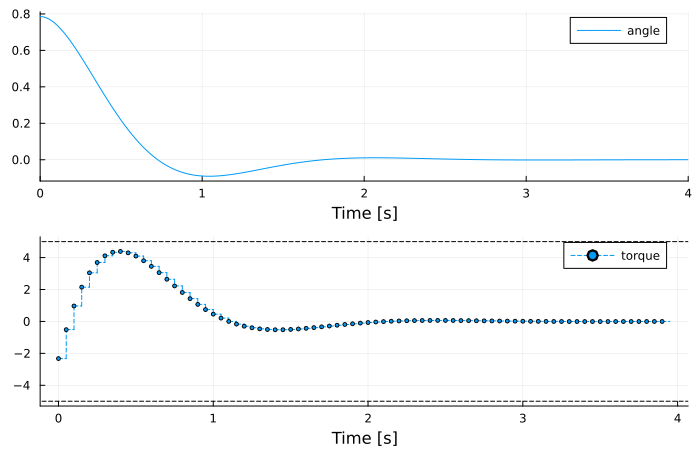
Gravity accelerates the pendulum toward the hanging position, and the controller applies a positive torque that limits the angular velocity, so that the pendulum comes to rest at the hanging position after a small overshoot. The torque peaks at about 4.4, just below the bound; with a tighter bound, the controller would instead hold the torque at the bound for a part of the motion. acados returns the status 0 at every sample instant.
The tutorials MPC with quadratic cost functions and MPC control of a Continuously Stirred Tank Reactor (CSTR) extend this example with reference tracking, state constraints, real-time iterations and a plant-model mismatch.
using Test
tk = 0:0.05:4
@test all(==(0), sol(tk, idxs = ssys.flag).u)
@test abs(sol(4.0, idxs = ssys.theta)) < 1e-2
@test maximum(abs, sol(tk, idxs = ssys.u1).u) <= 5 + 1e-6
Test Passed