

Analog.Examples.BridgeRectifier
Full-wave bridge rectifier with a capacitor-input filter.
Four Diodes fed from a floating sine source through a series resistance, into a smoothing capacitor and a resistive load. Diodes written anode -> cathode:
  d1: ac1 -> DC+        d3: GND -> ac1
d2: ac2 -> DC+ d4: GND -> ac2d1/d4 conduct on the half cycle where ac1 is the positive terminal, d2/d3 on the other, so the load sees both halves and the ripple is at 2*f_ac.
What this exercises
Four Diode2 junctions commutating twice per cycle, each swinging its small-signal conductance over many decades – from the crest of the charging burst down to blocking, where the exponential has saturated at -Ids and the only remaining path is the parallel Gp. The conduction angle is narrow because the capacitor holds DC+ near the peak: each diode conducts for a small fraction of the cycle and passes the whole load charge in a burst near the crest.
The output settles below the 17 V input peak by two forward drops plus the R_src and Rs drops at the charging peak. The expected values below are recorded from the run; re-record them if the card changes.
Why the extra parts
R_src is not optional. It stands for transformer secondary resistance. Driving a capacitor-input filter from an ideal voltage source leaves peak current limited only by the diodes' own Rs, which is both unphysical and badly conditioned.
Gp is load-bearing here, not a formality. The source is floating, so the ac1/ac2 pair has no galvanic path to ground – only the diodes' parallel conductances tie its common mode down. At the Diode2 default Gp = 1e-6 the run succeeds; at Gp = 0 the common mode is undetermined once all four diodes are off, and the integration fails. This is exactly what Gp is in the model for, and why Diode2 carries it while Diode uses a parallel R instead.
Breakdown is not reached. Reverse voltage never exceeds the 17 V peak, far below the Bv = 100 default, so the breakdown branch stays untaken. It is still evaluated – the three-region expression is one ifelse chain with no region tests – so it costs an exponential per evaluation regardless.
Validity
Diode has no charge model, so these diodes have no reverse recovery: they stop conducting the instant the junction voltage reverses. A real rectifier draws a reverse current spike at each commutation, which is a principal loss mechanism and the reason ultrafast parts exist. Switching loss from this circuit is therefore optimistic.
Solver notes
alg = ODEAlg.Rodas5P(), abstol = reltol = 1e-6. 6342 steps for the 250 ms span; stop scales the cost linearly. Tightening to 1e-8 takes 2.4x the steps and leaves the mean and ripple identical to five decimals, so 1e-6 is sufficient rather than merely tolerable.
Initial conditions
One differential state, the capacitor. The bridge also leaves one algebraic unknown – the floating common mode – for which Diode's own guess V = 0 suffices; giving it an initial value instead makes the initialization system overdetermined.
Usage
ElectricalComponents.Analog.Examples.BridgeRectifier(V_ac=17.0, f_ac=50.0, R_src=1.0, R_load=100.0, C_smooth=1u, Ids_d=2n, N_d=1.6, Rs_d=35m)
Parameters:
| Name | Description | Units | Default value |
|---|---|---|---|
V_ac | Peak input voltage, i.e. transformer secondary amplitude | V | 17.0 |
f_ac | Line frequency | Hz | 50.0 |
R_src | Source series resistance, standing for transformer secondary resistance | Ω | 1.0 |
R_load | Load resistance | Ω | 100.0 |
C_smooth | Reservoir capacitance | F | 1u |
Ids_d | Diode reverse saturation current | A | 2n |
N_d | Diode emission coefficient | – | 1.6 |
Rs_d | Diode ohmic series resistance | Ω | 35m |
Behavior
Source
"""
Full-wave bridge rectifier with a capacitor-input filter.

Four `Diode`s fed from a floating sine source through a series resistance, into a
smoothing capacitor and a resistive load.  Diodes written anode -> cathode:

```
  d1: ac1 -> DC+        d3: GND -> ac1
  d2: ac2 -> DC+        d4: GND -> ac2
```

`d1`/`d4` conduct on the half cycle where `ac1` is the positive terminal, `d2`/`d3`
on the other, so the load sees both halves and the ripple is at `2*f_ac`.

## What this exercises

Four `Diode2` junctions commutating twice per cycle, each swinging its
small-signal conductance over many decades -- from the crest of the charging
burst down to blocking, where the exponential has saturated at `-Ids` and the
only remaining path is the parallel `Gp`.  The conduction angle is narrow because
the capacitor holds `DC+` near the peak: each diode conducts for a small fraction
of the cycle and passes the whole load charge in a burst near the crest.

The output settles below the 17 V input peak by two forward drops plus the
`R_src` and `Rs` drops at the charging peak.  The expected values below are
recorded from the run; re-record them if the card changes.

## Why the extra parts

**`R_src` is not optional.** It stands for transformer secondary resistance.
Driving a capacitor-input filter from an ideal voltage source leaves peak current
limited only by the diodes' own `Rs`, which is both unphysical and badly
conditioned.

**`Gp` is load-bearing here, not a formality.** The source is floating, so the
`ac1`/`ac2` pair has no galvanic path to ground -- only the diodes' parallel
conductances tie its common mode down.  At the `Diode2` default `Gp = 1e-6` the
run succeeds; at `Gp = 0` the common mode is undetermined once all four diodes
are off, and the integration fails.  This is exactly what `Gp` is in the model
for, and why `Diode2` carries it while `Diode` uses a parallel `R` instead.

**Breakdown is not reached.**  Reverse voltage never exceeds the 17 V peak, far
below the `Bv = 100` default, so the breakdown branch stays untaken.  It is still
evaluated -- the three-region expression is one `ifelse` chain with no region
tests -- so it costs an exponential per evaluation regardless.

## Validity

`Diode` has no charge model, so these diodes have **no reverse recovery**: they
stop conducting the instant the junction voltage reverses.  A real rectifier
draws a reverse current spike at each commutation, which is a principal loss
mechanism and the reason ultrafast parts exist.  Switching loss from this
circuit is therefore optimistic.

## Solver notes

`alg = ODEAlg.Rodas5P()`, `abstol = reltol = 1e-6`.  6342 steps for the 250 ms
span; `stop` scales the cost linearly.  Tightening to 1e-8 takes 2.4x the steps
and leaves the mean and ripple identical to five decimals, so 1e-6 is sufficient
rather than merely tolerable.

## Initial conditions

One differential state, the capacitor.  The bridge also leaves **one algebraic
unknown** -- the floating common mode -- for which `Diode`'s own `guess V = 0`
suffices; giving it an initial value instead makes the initialization system
overdetermined.
"""
example component BridgeRectifier
  "Transformer secondary, floating"
  src = ElectricalComponents.Analog.Sources.VoltageSource() {
    "Dyad": {"placement": {"diagram": {"x1": 155, "x2": 255, "y1": 435, "y2": 535}}}
  }
  "Line waveform"
  sig = BlockComponents.Sources.Sine(amplitude = V_ac, frequency = f_ac) {
    "Dyad": {"placement": {"diagram": {"x1": 20, "x2": 120, "y1": 320, "y2": 420}}}
  }
  "Secondary resistance; see the note above on why this is required"
  rsrc = ElectricalComponents.Analog.Basic.Resistor(R = R_src) {
    "Dyad": {"placement": {"diagram": {"x1": 285, "x2": 385, "y1": 330, "y2": 430}}}
  }
  "ac1 -> DC+"
  d1 = ElectricalComponents.Analog.Semiconductors.Diode2(Ids = Ids_d, N = N_d, Rs = Rs_d) {
    "Dyad": {"placement": {"diagram": {"x1": 415, "x2": 515, "y1": 330, "y2": 430}}}
  }
  "ac2 -> DC+"
  d2 = ElectricalComponents.Analog.Semiconductors.Diode2(Ids = Ids_d, N = N_d, Rs = Rs_d) {
    "Dyad": {"placement": {"diagram": {"x1": 545, "x2": 645, "y1": 435, "y2": 535}}}
  }
  "GND -> ac1"
  d3 = ElectricalComponents.Analog.Semiconductors.Diode2(Ids = Ids_d, N = N_d, Rs = Rs_d) {
    "Dyad": {"placement": {"diagram": {"x1": 545, "x2": 645, "y1": 215, "y2": 315}}}
  }
  "GND -> ac2"
  d4 = ElectricalComponents.Analog.Semiconductors.Diode2(Ids = Ids_d, N = N_d, Rs = Rs_d) {
    "Dyad": {"placement": {"diagram": {"x1": 695, "x2": 795, "y1": 320, "y2": 420}}}
  }
  "Reservoir capacitor across the output"
  csmooth = ElectricalComponents.Analog.Basic.Capacitor(C = C_smooth) {
    "Dyad": {"placement": {"diagram": {"x1": 825, "x2": 925, "y1": 120, "y2": 220}}}
  }
  "Load"
  rload = ElectricalComponents.Analog.Basic.Resistor(R = R_load) {
    "Dyad": {"placement": {"diagram": {"x1": 955, "x2": 1055, "y1": 20, "y2": 120}}}
  }
  "Ground, at the negative output rail"
  ground = ElectricalComponents.Analog.Basic.Ground() {
    "Dyad": {"placement": {"diagram": {"x1": 1080, "x2": 1180, "y1": 95, "y2": 195}}}
  }
  "Peak input voltage, i.e. transformer secondary amplitude"
  parameter V_ac::Voltage = 17.0
  "Line frequency"
  parameter f_ac::Frequency = 50.0
  "Source series resistance, standing for transformer secondary resistance"
  parameter R_src::Resistance = 1.0
  "Load resistance"
  parameter R_load::Resistance = 100.0
  "Reservoir capacitance"
  parameter C_smooth::Capacitance = 1u
  "Diode reverse saturation current"
  parameter Ids_d::Current = 2n
  "Diode emission coefficient"
  parameter N_d::Real = 1.6
  "Diode ohmic series resistance"
  parameter Rs_d::Resistance = 35m
relations
  "One differential state, the reservoir capacitor, starting discharged"
  initial csmooth.v = 0
  connect(sig.y, src.V) {"Dyad": {"edges": [{"S": 1, "M": [{"x": 205, "y": 370}], "E": 2}], "path": {}}}
  connect(src.p, rsrc.p) {
    "Dyad": {
      "edges": [{"S": 1, "M": [{"x": 140, "y": 485}, {"x": 140, "y": 380}], "E": 2}],
      "path": {}
    }
  }
  "ac1: through the secondary resistance"
  connect(rsrc.n, d1.p, d3.n) {
    "Dyad": {
      "edges": [
        {"S": 1, "M": [], "E": -1},
        {"S": -1, "M": [], "E": 2},
        {
          "S": -1,
          "M": [{"x": 400, "y": 165}, {"x": 660, "y": 165}, {"x": 660, "y": 265}],
          "E": 3
        }
      ],
      "junctions": [{"x": 400, "y": 380}],
      "path": {}
    }
  }
  "ac2: the source return, floating"
  connect(src.n, d2.p, d4.n) {
    "Dyad": {
      "edges": [
        {"S": 1, "M": [], "E": -1},
        {"S": -1, "M": [], "E": 2},
        {
          "S": -1,
          "M": [{"x": 530, "y": 590}, {"x": 810, "y": 590}, {"x": 810, "y": 370}],
          "E": 3
        }
      ],
      "junctions": [{"x": 530, "y": 485}],
      "path": {}
    }
  }
  "DC+: upper diode cathodes, reservoir, load"
  connect(d1.n, d2.n, csmooth.p, rload.p) {
    "Dyad": {
      "edges": [
        {"S": 1, "M": [], "E": -1},
        {"S": -1, "M": [{"x": 670, "y": 485}], "E": 2},
        {"S": -1, "M": [{"x": 670, "y": 170}], "E": -2},
        {"S": -2, "M": [], "E": 3},
        {"S": -2, "M": [{"x": 810, "y": 70}], "E": 4}
      ],
      "junctions": [{"x": 670, "y": 380}, {"x": 810, "y": 170}],
      "path": {}
    }
  }
  "DC-: lower diode anodes, reservoir, load, and the only ground in the circuit"
  connect(d3.p, d4.p, csmooth.n, rload.n, ground.g) {
    "Dyad": {
      "edges": [
        {"S": 1, "M": [{"x": 530, "y": 265}, {"x": 530, "y": 370}], "E": -1},
        {"S": -1, "M": [], "E": 2},
        {"S": -1, "M": [{"x": 680, "y": 270}, {"x": 940, "y": 270}], "E": -2},
        {"S": -2, "M": [], "E": 3},
        {"S": -2, "M": [{"x": 1070, "y": 170}], "E": -3},
        {"S": -3, "M": [], "E": 4},
        {"S": -3, "M": [{"x": 1130, "y": 70}], "E": 5}
      ],
      "junctions": [{"x": 680, "y": 370}, {"x": 940, "y": 170}, {"x": 1070, "y": 70}],
      "path": {}
    }
  }
metadata {
  "Dyad": {
    "icons": {"default": "dyad://ElectricalComponents/Example.svg"},
    "tests": {
      "case1": {
        "solver": "Rodas5P",
        "stop": 0.25,
        "abstol": 0.000001,
        "reltol": 0.000001,
        "expect": {"signals": ["csmooth.v", "d1.i"]}
      }
    }
  }
}
end
Flattened Source
"""
Full-wave bridge rectifier with a capacitor-input filter.

Four `Diode`s fed from a floating sine source through a series resistance, into a
smoothing capacitor and a resistive load.  Diodes written anode -> cathode:

```
  d1: ac1 -> DC+        d3: GND -> ac1
  d2: ac2 -> DC+        d4: GND -> ac2
```

`d1`/`d4` conduct on the half cycle where `ac1` is the positive terminal, `d2`/`d3`
on the other, so the load sees both halves and the ripple is at `2*f_ac`.

## What this exercises

Four `Diode2` junctions commutating twice per cycle, each swinging its
small-signal conductance over many decades -- from the crest of the charging
burst down to blocking, where the exponential has saturated at `-Ids` and the
only remaining path is the parallel `Gp`.  The conduction angle is narrow because
the capacitor holds `DC+` near the peak: each diode conducts for a small fraction
of the cycle and passes the whole load charge in a burst near the crest.

The output settles below the 17 V input peak by two forward drops plus the
`R_src` and `Rs` drops at the charging peak.  The expected values below are
recorded from the run; re-record them if the card changes.

## Why the extra parts

**`R_src` is not optional.** It stands for transformer secondary resistance.
Driving a capacitor-input filter from an ideal voltage source leaves peak current
limited only by the diodes' own `Rs`, which is both unphysical and badly
conditioned.

**`Gp` is load-bearing here, not a formality.** The source is floating, so the
`ac1`/`ac2` pair has no galvanic path to ground -- only the diodes' parallel
conductances tie its common mode down.  At the `Diode2` default `Gp = 1e-6` the
run succeeds; at `Gp = 0` the common mode is undetermined once all four diodes
are off, and the integration fails.  This is exactly what `Gp` is in the model
for, and why `Diode2` carries it while `Diode` uses a parallel `R` instead.

**Breakdown is not reached.**  Reverse voltage never exceeds the 17 V peak, far
below the `Bv = 100` default, so the breakdown branch stays untaken.  It is still
evaluated -- the three-region expression is one `ifelse` chain with no region
tests -- so it costs an exponential per evaluation regardless.

## Validity

`Diode` has no charge model, so these diodes have **no reverse recovery**: they
stop conducting the instant the junction voltage reverses.  A real rectifier
draws a reverse current spike at each commutation, which is a principal loss
mechanism and the reason ultrafast parts exist.  Switching loss from this
circuit is therefore optimistic.

## Solver notes

`alg = ODEAlg.Rodas5P()`, `abstol = reltol = 1e-6`.  6342 steps for the 250 ms
span; `stop` scales the cost linearly.  Tightening to 1e-8 takes 2.4x the steps
and leaves the mean and ripple identical to five decimals, so 1e-6 is sufficient
rather than merely tolerable.

## Initial conditions

One differential state, the capacitor.  The bridge also leaves **one algebraic
unknown** -- the floating common mode -- for which `Diode`'s own `guess V = 0`
suffices; giving it an initial value instead makes the initialization system
overdetermined.
"""
example component BridgeRectifier
  "Transformer secondary, floating"
  src = ElectricalComponents.Analog.Sources.VoltageSource() {
    "Dyad": {"placement": {"diagram": {"x1": 155, "x2": 255, "y1": 435, "y2": 535}}}
  }
  "Line waveform"
  sig = BlockComponents.Sources.Sine(amplitude = V_ac, frequency = f_ac) {
    "Dyad": {"placement": {"diagram": {"x1": 20, "x2": 120, "y1": 320, "y2": 420}}}
  }
  "Secondary resistance; see the note above on why this is required"
  rsrc = ElectricalComponents.Analog.Basic.Resistor(R = R_src) {
    "Dyad": {"placement": {"diagram": {"x1": 285, "x2": 385, "y1": 330, "y2": 430}}}
  }
  "ac1 -> DC+"
  d1 = ElectricalComponents.Analog.Semiconductors.Diode2(Ids = Ids_d, N = N_d, Rs = Rs_d) {
    "Dyad": {"placement": {"diagram": {"x1": 415, "x2": 515, "y1": 330, "y2": 430}}}
  }
  "ac2 -> DC+"
  d2 = ElectricalComponents.Analog.Semiconductors.Diode2(Ids = Ids_d, N = N_d, Rs = Rs_d) {
    "Dyad": {"placement": {"diagram": {"x1": 545, "x2": 645, "y1": 435, "y2": 535}}}
  }
  "GND -> ac1"
  d3 = ElectricalComponents.Analog.Semiconductors.Diode2(Ids = Ids_d, N = N_d, Rs = Rs_d) {
    "Dyad": {"placement": {"diagram": {"x1": 545, "x2": 645, "y1": 215, "y2": 315}}}
  }
  "GND -> ac2"
  d4 = ElectricalComponents.Analog.Semiconductors.Diode2(Ids = Ids_d, N = N_d, Rs = Rs_d) {
    "Dyad": {"placement": {"diagram": {"x1": 695, "x2": 795, "y1": 320, "y2": 420}}}
  }
  "Reservoir capacitor across the output"
  csmooth = ElectricalComponents.Analog.Basic.Capacitor(C = C_smooth) {
    "Dyad": {"placement": {"diagram": {"x1": 825, "x2": 925, "y1": 120, "y2": 220}}}
  }
  "Load"
  rload = ElectricalComponents.Analog.Basic.Resistor(R = R_load) {
    "Dyad": {"placement": {"diagram": {"x1": 955, "x2": 1055, "y1": 20, "y2": 120}}}
  }
  "Ground, at the negative output rail"
  ground = ElectricalComponents.Analog.Basic.Ground() {
    "Dyad": {"placement": {"diagram": {"x1": 1080, "x2": 1180, "y1": 95, "y2": 195}}}
  }
  "Peak input voltage, i.e. transformer secondary amplitude"
  parameter V_ac::Voltage = 17.0
  "Line frequency"
  parameter f_ac::Frequency = 50.0
  "Source series resistance, standing for transformer secondary resistance"
  parameter R_src::Resistance = 1.0
  "Load resistance"
  parameter R_load::Resistance = 100.0
  "Reservoir capacitance"
  parameter C_smooth::Capacitance = 1u
  "Diode reverse saturation current"
  parameter Ids_d::Current = 2n
  "Diode emission coefficient"
  parameter N_d::Real = 1.6
  "Diode ohmic series resistance"
  parameter Rs_d::Resistance = 35m
relations
  "One differential state, the reservoir capacitor, starting discharged"
  initial csmooth.v = 0
  connect(sig.y, src.V) {"Dyad": {"edges": [{"S": 1, "M": [{"x": 205, "y": 370}], "E": 2}], "path": {}}}
  connect(src.p, rsrc.p) {
    "Dyad": {
      "edges": [{"S": 1, "M": [{"x": 140, "y": 485}, {"x": 140, "y": 380}], "E": 2}],
      "path": {}
    }
  }
  "ac1: through the secondary resistance"
  connect(rsrc.n, d1.p, d3.n) {
    "Dyad": {
      "edges": [
        {"S": 1, "M": [], "E": -1},
        {"S": -1, "M": [], "E": 2},
        {
          "S": -1,
          "M": [{"x": 400, "y": 165}, {"x": 660, "y": 165}, {"x": 660, "y": 265}],
          "E": 3
        }
      ],
      "junctions": [{"x": 400, "y": 380}],
      "path": {}
    }
  }
  "ac2: the source return, floating"
  connect(src.n, d2.p, d4.n) {
    "Dyad": {
      "edges": [
        {"S": 1, "M": [], "E": -1},
        {"S": -1, "M": [], "E": 2},
        {
          "S": -1,
          "M": [{"x": 530, "y": 590}, {"x": 810, "y": 590}, {"x": 810, "y": 370}],
          "E": 3
        }
      ],
      "junctions": [{"x": 530, "y": 485}],
      "path": {}
    }
  }
  "DC+: upper diode cathodes, reservoir, load"
  connect(d1.n, d2.n, csmooth.p, rload.p) {
    "Dyad": {
      "edges": [
        {"S": 1, "M": [], "E": -1},
        {"S": -1, "M": [{"x": 670, "y": 485}], "E": 2},
        {"S": -1, "M": [{"x": 670, "y": 170}], "E": -2},
        {"S": -2, "M": [], "E": 3},
        {"S": -2, "M": [{"x": 810, "y": 70}], "E": 4}
      ],
      "junctions": [{"x": 670, "y": 380}, {"x": 810, "y": 170}],
      "path": {}
    }
  }
  "DC-: lower diode anodes, reservoir, load, and the only ground in the circuit"
  connect(d3.p, d4.p, csmooth.n, rload.n, ground.g) {
    "Dyad": {
      "edges": [
        {"S": 1, "M": [{"x": 530, "y": 265}, {"x": 530, "y": 370}], "E": -1},
        {"S": -1, "M": [], "E": 2},
        {"S": -1, "M": [{"x": 680, "y": 270}, {"x": 940, "y": 270}], "E": -2},
        {"S": -2, "M": [], "E": 3},
        {"S": -2, "M": [{"x": 1070, "y": 170}], "E": -3},
        {"S": -3, "M": [], "E": 4},
        {"S": -3, "M": [{"x": 1130, "y": 70}], "E": 5}
      ],
      "junctions": [{"x": 680, "y": 370}, {"x": 940, "y": 170}, {"x": 1070, "y": 70}],
      "path": {}
    }
  }
metadata {
  "Dyad": {
    "icons": {"default": "dyad://ElectricalComponents/Example.svg"},
    "tests": {
      "case1": {
        "solver": "Rodas5P",
        "stop": 0.25,
        "abstol": 0.000001,
        "reltol": 0.000001,
        "expect": {"signals": ["csmooth.v", "d1.i"]}
      }
    }
  }
}
end
Test Cases
Test Case case1
plt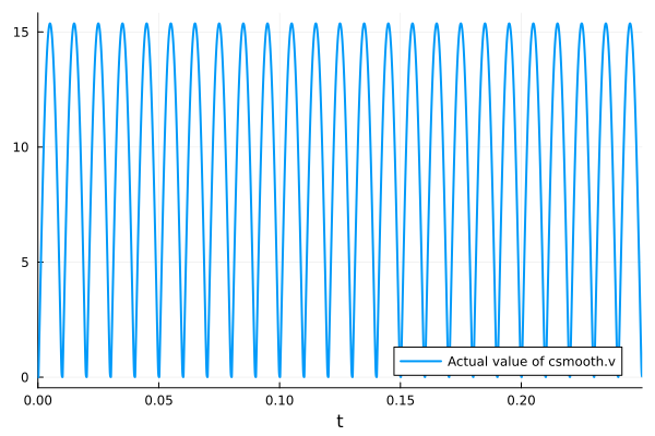
plt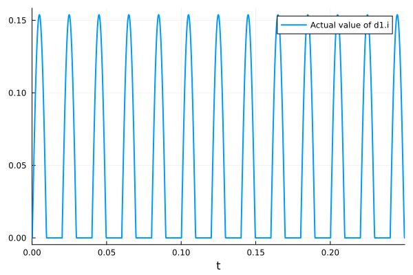
Related
Examples
Experiments
Analyses