
Download as a Dyad projectMPCIntroduction.zipOpen in Dyad Studio
Model-predictive control
Model-predictive control (MPC) uses a model of the controlled system to predict its response over a finite time interval, the prediction horizon, and an optimizer to compute the control signal over this interval that minimizes a cost function subject to constraints. At every sample instant the controller
estimates the current state of the system from the measurements,
solves the optimal-control problem over the prediction horizon, starting from this estimate,
applies the first control signal of the optimal sequence and discards the remainder.
At the next sample instant the procedure is repeated with a new measurement and a horizon that has moved forward by one sample. This is the receding-horizon principle. Since the optimization is repeated with new measurements, the controller is a feedback controller: model errors and disturbances that cause the system to deviate from the prediction are corrected at the following sample instants.
This page introduces the concepts that are common to both MPC controllers of this library. The formulation of each controller, i.e., its prediction model, cost function and constraints, is described on the pages Linear MPC and Nonlinear MPC.
Signals of an MPC loop
An MPC controller is a sampled-data controller connected to a continuous-time plant through samplers and holds:
              d (unmeasured)
                    │
   r ──►┌─────┐ u   ▼   ┌───────┐   y
   w ──►│ MPC ├──►[ZOH]─►│ Plant ├──►[Sampler]──┐
        └──▲──┘          └───────┘              │
           │  x̂       ┌──────────┐              │
           └──────────┤ Observer │◄─────────────┘
└──────────┘| Signal | Meaning |
|---|---|
| control signal, the decision variable of the optimization | |
| measured outputs, used by the observer to estimate the state | |
| state estimate, the initial state of the prediction | |
| reference for the controlled outputs, a constant or a trajectory over the horizon (preview) | |
| measured or known disturbances, e.g., a forecast, used in the prediction | |
| unmeasured disturbances, which the observer may estimate when they are included in the model |
The controlled outputs, which the cost function penalizes, and the constrained outputs need not coincide with the measured outputs. In MPCComponents the controllers are clocked components: the clock is provided by a PeriodicClock of DiscreteComponents, the measurements are sampled by Sampler components, and the control signal is held constant between samples by a ZeroOrderHold. The controller computes the control signal of a sample instant from the measurements of the same instant, i.e., the computation is assumed to take negligible time compared with the sample interval.
LinearMPCController contains the observer, a Kalman filter, and has the measurements y as its input. ACADOSMPC has the state x as its input; it is connected either directly to the sampled state variables or to an observer such as UKFObserver.
Why MPC?
Comparison with LQR control
The widely used linear-quadratic regulator (LQR) minimizes a quadratic cost over an infinite horizon for a linear model without constraints. The resulting controller is a constant state-feedback gain. Linear MPC with the same weights and a terminal cost equal to the infinite-horizon LQR cost-to-go coincides with the LQR controller as long as no constraint is active. The two controllers differ when the system operates at its limits:
Constraints. Actuators saturate, and variables such as velocities, temperatures or levels are subject to limits. The LQR controller is unaware of these limits. If its control signal is clipped, the closed-loop system no longer behaves as designed, which typically causes overshoot and may cause instability. MPC includes the limits in the optimization, and computes the best control signal that satisfies them.
Preview. MPC can use known future values of the reference and of disturbances, e.g., a planned trajectory, a weather forecast or a price signal, and act before they occur.
General objectives. The cost function may contain terms other than quadratic tracking errors, e.g., a linear energy cost in economic MPC (see Economic MPC for residential HVAC).
Nonlinear models. Nonlinear MPC uses a nonlinear model, which remains valid over a larger operating range than a linearization.
The following example compares a saturated LQR controller with an MPC controller on a double integrator, a unit mass driven by a force LinearMPCController without constraints and with the LQR cost-to-go as terminal cost (terminal_lqr_cost = true); its control signal is clipped by a Limiter. The MPC controller additionally contains the force bound and the velocity bound ymin, ymax) is set to a large value, so that only the bound on the velocity is active.
"""
Double integrator: a unit mass on a frictionless surface, driven by the force `u`. The state
consists of the position `x` and the velocity `v`, both of which are available as outputs.
"""
component DoubleIntegratorPlant
  "Force"
  u = RealInput() {^u}
  "Position"
  position = RealOutput() {^position}
  "Velocity"
  velocity = RealOutput() {^velocity}
  "Mass"
  parameter m::Real = 1.0
  "Initial position"
  parameter x0::Real = 0.0
  "Initial velocity"
  parameter v0::Real = 0.0
  "Position"
  variable x::Real(initial = x0)
  "Velocity"
  variable v::Real(initial = v0)
relations
  der(x) = v
  m * der(v) = u
  position = x
  velocity = v
metadata {
  "Dyad": {
    "icons": {"default": "dyad://MPCComponents/DoubleIntegratorExamplePlant.svg"},
    "doc": {"behavior": false}
  },
  "_links": {
    "u": {
      "Dyad": {"placement": {"diagram": {"x1": -100, "x2": 0, "y1": 450, "y2": 550}}}
    },
    "position": {
      "Dyad": {"placement": {"diagram": {"x1": 1000, "x2": 1100, "y1": 250, "y2": 350}}}
    },
    "velocity": {
      "Dyad": {"placement": {"diagram": {"x1": 1000, "x2": 1100, "y1": 650, "y2": 750}}}
    }
  }
}
end

"""
Comparison of a saturated LQR controller with an MPC controller on the double integrator
`DoubleIntegratorPlant`, both regulating the position from -2 to the origin with the full state
measured. The force is limited to ``|u| \\le`` `umax`.

The first loop uses an unconstrained `LinearMPCController` with the LQR cost-to-go as terminal cost,
which coincides with the LQR controller, followed by a `Limiter` at the plant input. The controller is
unaware of the saturation. The second loop uses the same weights, with the force bound and the velocity
bound ``|v| \\le`` `vmax` given to the controller as constraints.
"""
example component SaturatedLQRvsMPCExample
  "Force bound"
  structural parameter umax::Real = 1.0
  "Velocity bound of the MPC controller"
  structural parameter vmax::Real = 0.8
  clock_lqr = DiscreteComponents.PeriodicClock(dt = 0.1) {^clock_lqr}
  clock_mpc = DiscreteComponents.PeriodicClock(dt = 0.1) {^clock_mpc}
  plant_lqr = DoubleIntegratorPlant(x0 = -2.0) {^plant_lqr}
  plant_mpc = DoubleIntegratorPlant(x0 = -2.0) {^plant_mpc}
  sx_lqr = DiscreteComponents.Sampler() {^sx_lqr}
  sv_lqr = DiscreteComponents.Sampler() {^sv_lqr}
  sx_mpc = DiscreteComponents.Sampler() {^sx_mpc}
  sv_mpc = DiscreteComponents.Sampler() {^sv_mpc}
  zoh_lqr = DiscreteComponents.ZeroOrderHold() {^zoh_lqr}
  zoh_mpc = DiscreteComponents.ZeroOrderHold() {^zoh_mpc}
  saturation = BlockComponents.Nonlinear.Limiter(final y_max = umax) {^saturation}
  lqr = MPCComponents.LinearMPCController(dynamics = plant_lqr, inputs = ["u"], outputs = ["position", "velocity"], state_variables = ["x", "v"], Ts = 0.1, Np = 50, Q1 = [1.0, 0.0], Q2 = [0.01], reference_tracking = false, terminal_lqr_cost = true, R1 = [1.0, 1.0], R2 = [1e-6, 1e-6]) {^lqr}
  mpc = MPCComponents.LinearMPCController(dynamics = plant_mpc, inputs = ["u"], outputs = ["position", "velocity"], state_variables = ["x", "v"], Ts = 0.1, Np = 50, Q1 = [1.0, 0.0], Q2 = [0.01], reference_tracking = false, terminal_lqr_cost = true, umin = [-umax], umax = [umax], ymin = [-1e3, -vmax], ymax = [1e3, vmax], R1 = [1.0, 1.0], R2 = [1e-6, 1e-6]) {^mpc}
  "Position with the saturated LQR controller"
  variable x_lqr::Real
  "Velocity with the saturated LQR controller"
  variable v_lqr::Real
  "Force with the saturated LQR controller (after the limiter)"
  variable u_lqr::Real
  "Position with the MPC controller"
  variable x_mpc::Real
  "Velocity with the MPC controller"
  variable v_mpc::Real
  "Force with the MPC controller"
  variable u_mpc::Real
relations
  x_lqr = plant_lqr.position
  v_lqr = plant_lqr.velocity
  u_lqr = saturation.y
  x_mpc = plant_mpc.position
  v_mpc = plant_mpc.velocity
  u_mpc = zoh_mpc.y
  connect(plant_lqr.position, sx_lqr.u)
  connect(plant_lqr.velocity, sv_lqr.u)
  connect(sx_lqr.y, lqr.y[1], clock_lqr.y)
  connect(sv_lqr.y, lqr.y[2])
  connect(lqr.u[1], zoh_lqr.u)
  connect(zoh_lqr.y, saturation.u)
  connect(saturation.y, plant_lqr.u)
  connect(plant_mpc.position, sx_mpc.u)
  connect(plant_mpc.velocity, sv_mpc.u)
  connect(sx_mpc.y, mpc.y[1], clock_mpc.y)
  connect(sv_mpc.y, mpc.y[2])
  connect(mpc.u[1], zoh_mpc.u)
  connect(zoh_mpc.y, plant_mpc.u)
metadata {
  "Dyad": {"doc": {"behavior": false}},
  "_links": {
    "clock_lqr": {},
    "clock_mpc": {},
    "plant_lqr": {},
    "plant_mpc": {},
    "sx_lqr": {},
    "sv_lqr": {},
    "sx_mpc": {},
    "sv_mpc": {},
    "zoh_lqr": {},
    "zoh_mpc": {},
    "saturation": {},
    "lqr": {},
    "mpc": {}
  }
}
end
Both state variables are measured, and the measurement noise covariance R2 is small compared with the process noise covariance R1, so the Kalman filters of the two controllers reproduce the measured state.
@named model = SaturatedLQRvsMPCExample()
ssys = mtkcompile(model; additional_passes = [SynchToolkit.compile_lustre])
prob = ODEProblem(ssys, [], (0.0, 10.0))
sol = solve(prob)
plot(sol, idxs = [ssys.x_lqr, ssys.x_mpc, ssys.v_lqr, ssys.v_mpc, ssys.u_lqr, ssys.u_mpc],
     layout = (3, 1), sp = [1 1 2 2 3 3], lab = ["saturated LQR" "MPC" "" "" "" ""],
     ylabel = ["position" "velocity" "force"], xlabel = "Time [s]", size = (700, 600))
hline!([0.8], sp = 2, l = (:black, :dash), lab = "")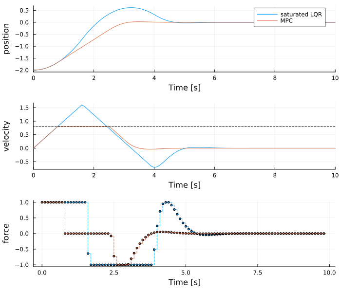
The LQR gain is designed for small deviations, and the initial deviation of 2 causes a control signal far beyond the force bound. The clipped control signal accelerates the mass for a longer time than the LQR design assumes, and the controller starts to decelerate too late, so the position overshoots the target by about 0.6. The MPC controller predicts that the force is bounded, accelerates to the velocity bound, and starts to decelerate in time to reach the target without significant overshoot.
Comparison with PID control
PID controllers are the most common controllers in industry. They require no model and have few parameters. MPC is preferable when
the system has several inputs and outputs with significant coupling, which a set of single-loop PID controllers handles poorly,
constraints on inputs, rates of change and outputs determine the achievable performance,
the system has long time delays or non-minimum-phase dynamics, which a model-based prediction handles directly,
future references or disturbances are known in advance.
The component PIDEquivalentMPCController is a linear MPC controller that reproduces a discrete-time PID controller exactly as long as no constraint is active. It allows constraints and preview to be added to an existing, tuned PID controller. This controller may be used as a drop-in replacement of a PID controller that keeps the same tuning parameters, but enable some of the advanced features offered by MPC controllers.
Costs of MPC
These advantages come at a cost:
MPC requires a model of the system, and the performance depends on its accuracy. If you have implemented a simulation model in Dyad, this model may be used by the MPC.
An optimization problem is solved at every sample instant. For linear MPC, the computation time is typically in the range of microseconds to milliseconds; for nonlinear MPC or when using binary input variables, it may be considerably larger, and the solver may fail to converge.
A state estimator (observer) is required.
The behavior of the closed-loop system is determined by more parameters than for PID control: weights, horizons, constraints and the estimator.
Linear or nonlinear MPC
MPCComponents provides two MPC controllers.
LinearMPCControlleruses a linear, discrete-time prediction model and a quadratic cost function. The optimization problem is a quadratic program (QP), which is condensed when the model is built and solved by the QP solver DAQP at every sample instant. The prediction model is either given as matrices or obtained by automatic linearization of a Dyad plant model. The controller contains a Kalman filter. See Linear MPC.ACADOSMPCuses a nonlinear, continuous-time prediction model, given as a Dyad plant model, and solves a nonlinear optimal-control problem with the sequential quadratic programming (SQP) solver of acados. See Nonlinear MPC.
| Linear MPC is preferable when | Nonlinear MPC is preferable when |
|---|---|
| a single linearization predicts the plant well in the operating range, or the response is determined mainly by the bounds | the plant operates over a large range with significant changes of its dynamics |
| the computation time must be as small as possible or deterministic | the constraints or the cost function are nonlinear in the state |
| binary or integer control signals are required | plant parameters change online |
| the cost function contains linear economic terms | the error of the linear model exceeds what the disturbance estimate compensates |
Both controllers can be exported to standalone C code together with the rest of a discrete-time model, with the analysis CCodeExport.
Further reading
Linear MPC and Nonlinear MPC describe the formulation of each controller, with a basic example.
The tutorials demonstrate both controllers on a range of applications, starting with MPC with quadratic cost functions and Disturbance modeling and rejection with MPC controllers.
using Test
@test sol(10.0, idxs = ssys.x_mpc) ≈ 0 atol = 1e-4
@test maximum(sol[ssys.x_lqr]) > 0.5
@test maximum(sol[ssys.x_mpc]) < 0.05
@test maximum(abs, sol[ssys.v_mpc]) < 0.8 + 1e-3
@test maximum(abs, sol[ssys.u_mpc]) <= 1 + 1e-9
Test Passed