
MPC with binary or integer variables (MINLP)
This example demonstrates how to solve MPC problems where some variables are constrained to be binary or integer valued (a binary variable is a special case of an integer variable). A common situation where such constraints arise is when an actuator can be either on or off, but nothing in between. Examples of situations in which integer-valued variables are useful
Compressors without inverter control can only be on or off, but not in between.
Thermostats often operate in an on-off fashion.
Actuators controlled through relays or switches.
Actuators with a significant cost associated with switching on or off, such as power plants.
Discrete choices, such as selecting between different modes of operation.
Optimization with a mix of integer and real variables is often referred to as "mixed-integer nonlinear programming" (MINLP), so we are in this tutorial solving what is referred to as an MINLP MPC problem. Since the plant below is linear and the cost is quadratic, the optimization problem is in this case a mixed-integer quadratic program (MIQP).
In this example, we will consider a simple double integrator, but constrain the input
We start by defining the dynamics and the cost. The plant is the discrete-time state-space model DiscreteComponents.DiscreteStateSpace with the sample time C is the identity matrix):
plant1 = DiscreteComponents.DiscreteStateSpace(nx = 2, nu = 1, ny = 2, A = [[1.0, 0.1], [0.0, 1.0]], B = [[0.0], [0.1]], C = [[1.0, 0.0], [0.0, 1.0]], with_D = false, initialization = DiscreteComponents.InitialCondition.InitialStateArray(x0 = [10.0, 0.0]))The controller is a LinearMPCOptimizer, whose MPC problem is built by build_linear_mpc from the same model. The MPC optimization horizon is Np = 10, the state cost has unit weight on both state components (Q1), the control cost is Q2), and the terminal cost has ten times the weight of the state cost (Qf). The reference is zero, which reference_tracking = false expresses by regulating to the origin:
build_linear_mpc(A = [[1.0, 0.1], [0.0, 1.0]], B = [[0.0], [0.1]], Np = 10, Q1 = [1.0, 1.0], Q2 = [0.1], Qf = [10.0, 10.0], umin = [-1.0], umax = [1.0], reference_tracking = false)We then define the constraints, here, we constrain the control input to be between umin and umax above. We will constrain y directly to the state input xhat of the optimizer, i.e., the controller does not use an observer, it knows the state of the system from the simulation model.
When we define the solver, there is nothing to choose in this case: LinearMPC.jl condenses the MPC problem into a quadratic program that is solved by the active-set solver DAQP, and when some control inputs are binary, DAQP solves the resulting mixed-integer quadratic program by branch and bound.
To indicate that the control input is integer valued, we provide the parameter binary_controls. This is a vector with the indices of the control inputs that are restricted to the two values {umin, umax}. A binary control can thus take only two values, and we encode the three-valued integer set by two binary inputs, Q2, which keeps the Hessian of the MIQP positive definite and makes
build_linear_mpc(A = [[1.0, 0.1], [0.0, 1.0]], B = [[0.0, 0.0], [0.1, -0.1]], Np = 10, Q1 = [1.0, 1.0], Q2 = [[0.100001, -0.1], [-0.1, 0.100001]], Qf = [10.0, 10.0], umin = [0.0, 0.0], umax = [1.0, 1.0], binary_controls = [1, 2], reference_tracking = false)The model below contains three parallel closed loops around the same plant, which we will compare in this tutorial: real-valued control (plant1, mpc1), integer-valued control over the full horizon (plant2, mpc2), and integer-valued control over part of the horizon (plant3, mpc3), which we discuss in the section Speed up computation below. The variables p, v and u of each loop make the position, the velocity and the control signal available for plotting, with u2 = mpc2.u[1] - mpc2.u[2] for the integer-valued loops.
"""
Regulation of a double integrator to the origin with the control restricted to the integer
values `u ∈ {-1, 0, 1}` — the Dyad version of the DyadControlSystems MINLP MPC tutorial
(https://help.juliahub.com/dyad/DyadControlSystems.jl/stable/examples/minlp_mpc/). Three
parallel closed loops around the same plant from the initial state `[10, 0]` compare real-valued control (loop 1), integer control enforced
over the full horizon (loop 2), and integer control enforced over only the first two prediction
steps (loop 3, `Nc_binary = 2` — the tutorial's `Nint`). The plants are exact discrete models
(`DiscreteStateSpace`) and the full state is fed to a `LinearMPCOptimizer` directly, the Dyad
version of the tutorial's `StateFeedback` observer. The cost is the tutorial's:
unit weight on both states, `0.1 u^2` on the control and ten times the state weight as terminal
cost.

DAQP's binary controls take only the two values `{umin, umax}`, so the three-valued integer set
is encoded with two binary inputs `u = u1 - u2`, `u1, u2 ∈ {0, 1}`: the integer-controlled
plants take both inputs with input matrix `[B, -B]`, and the control weight is the rank-one
`0.1 (u1 - u2)^2` plus `1e-6` on the diagonal, which keeps the MIQP Hessian positive definite
and makes `(0, 0)` the preferred encoding of `u = 0`.
"""
example component IntegerControlMPCExample
  clock1 = DiscreteComponents.PeriodicClock(dt = 0.1) {^clock1}
  "Plant with real-valued control"
  plant1 = DiscreteComponents.DiscreteStateSpace(nx = 2, nu = 1, ny = 2, A = [[1.0, 0.1], [0.0, 1.0]], B = [[0.0], [0.1]], C = [[1.0, 0.0], [0.0, 1.0]], with_D = false, initialization = DiscreteComponents.InitialCondition.InitialStateArray(x0 = [10.0, 0.0])) {^plant1}
  "Real-valued MPC"
  mpc1 = MPCComponents.LinearMPCOptimizer(mpc = ctrl_real) {^mpc1}
  "Continuous-time hold of the control; a model with no continuous part fails to initialize"
  zoh1 = DiscreteComponents.ZeroOrderHold() {^zoh1}
  "Plant with integer control, u = u1 - u2"
  plant2 = DiscreteComponents.DiscreteStateSpace(nx = 2, nu = 2, ny = 2, A = [[1.0, 0.1], [0.0, 1.0]], B = [[0.0, 0.0], [0.1, -0.1]], C = [[1.0, 0.0], [0.0, 1.0]], with_D = false, initialization = DiscreteComponents.InitialCondition.InitialStateArray(x0 = [10.0, 0.0])) {^plant2}
  "MPC with binary controls over the full horizon"
  mpc2 = MPCComponents.LinearMPCOptimizer(mpc = ctrl_binary) {^mpc2}
  "Continuous-time hold of the control; a model with no continuous part fails to initialize"
  zoh2 = DiscreteComponents.ZeroOrderHold() {^zoh2}
  "Plant with integer control, u = u1 - u2"
  plant3 = DiscreteComponents.DiscreteStateSpace(nx = 2, nu = 2, ny = 2, A = [[1.0, 0.1], [0.0, 1.0]], B = [[0.0, 0.0], [0.1, -0.1]], C = [[1.0, 0.0], [0.0, 1.0]], with_D = false, initialization = DiscreteComponents.InitialCondition.InitialStateArray(x0 = [10.0, 0.0])) {^plant3}
  "MPC with binary controls over the first two prediction steps only"
  mpc3 = MPCComponents.LinearMPCOptimizer(mpc = ctrl_binary2) {^mpc3}
  "Continuous-time hold of the control; a model with no continuous part fails to initialize"
  zoh3 = DiscreteComponents.ZeroOrderHold() {^zoh3}
  periodicclock = DiscreteComponents.PeriodicClock(dt = 0.1) {^periodicclock}
  periodicclock1 = DiscreteComponents.PeriodicClock(dt = 0.1) {^periodicclock1}
  "Real-valued controller, u ∈ [-1, 1]"
  structural parameter ctrl_real::MPCComponents.MPCRef = build_linear_mpc(A = [[1.0, 0.1], [0.0, 1.0]], B = [[0.0], [0.1]], Np = 10, Q1 = [1.0, 1.0], Q2 = [0.1], Qf = [10.0, 10.0], umin = [-1.0], umax = [1.0], reference_tracking = false)
  "Integer controller, u1 - u2 ∈ {-1, 0, 1} over the full horizon"
  structural parameter ctrl_binary::MPCComponents.MPCRef = build_linear_mpc(A = [[1.0, 0.1], [0.0, 1.0]], B = [[0.0, 0.0], [0.1, -0.1]], Np = 10, Q1 = [1.0, 1.0], Q2 = [[0.100001, -0.1], [-0.1, 0.100001]], Qf = [10.0, 10.0], umin = [0.0, 0.0], umax = [1.0, 1.0], binary_controls = [1, 2], reference_tracking = false)
  "Integer controller, binary only over the first two steps, relaxed to [0, 1] after"
  structural parameter ctrl_binary2::MPCComponents.MPCRef = build_linear_mpc(A = [[1.0, 0.1], [0.0, 1.0]], B = [[0.0, 0.0], [0.1, -0.1]], Np = 10, Q1 = [1.0, 1.0], Q2 = [[0.100001, -0.1], [-0.1, 0.100001]], Qf = [10.0, 10.0], umin = [0.0, 0.0], umax = [1.0, 1.0], binary_controls = [1, 2], Nc_binary = 2, reference_tracking = false)
  "Position, real-valued control"
  variable p1::Real
  "Velocity, real-valued control"
  variable v1::Real
  "Control signal, real-valued"
  variable u1::Real
  "Position, full binary horizon"
  variable p2::Real
  "Velocity, full binary horizon"
  variable v2::Real
  "Control signal u1 - u2, full binary horizon"
  variable u2::Real
  "Position, binary horizon 2"
  variable p3::Real
  "Velocity, binary horizon 2"
  variable v3::Real
  "Control signal u1 - u2, binary horizon 2"
  variable u3::Real
relations
  p1 = plant1.y[1]
  v1 = plant1.y[2]
  u1 = mpc1.u[1]
  p2 = plant2.y[1]
  v2 = plant2.y[2]
  u2 = mpc2.u[1] - mpc2.u[2]
  p3 = plant3.y[1]
  v3 = plant3.y[2]
  u3 = mpc3.u[1] - mpc3.u[2]
  connect(mpc1.u[1], zoh1.u, clock1.y) {^id13}
  connect(mpc2.u[1], zoh2.u, periodicclock.y) {^id14}
  connect(mpc3.u[1], zoh3.u, periodicclock1.y) {^id15}
  connect(plant1.y, mpc1.xhat) {^id16}
  connect(plant2.y, mpc2.xhat) {^id17}
  connect(mpc3.xhat, plant3.y) {^id18}
  connect(mpc1.u, plant1.u) {^id19}
  connect(mpc2.u, plant2.u) {^id20}
  connect(mpc3.u, plant3.u) {^id21}
metadata {
  "Dyad": {"doc": {"behavior": false}},
  "_links": {
    "clock1": {
      "Dyad": {"placement": {"diagram": {"x1": 530, "x2": 630, "y1": 70, "y2": 170}}}
    },
    "plant1": {
      "Dyad": {"placement": {"diagram": {"x1": 340, "x2": 440, "y1": 40, "y2": 140}}}
    },
    "mpc1": {
      "Dyad": {"placement": {"diagram": {"x1": 180, "x2": 280, "y1": 40, "y2": 140}}}
    },
    "zoh1": {
      "Dyad": {"placement": {"diagram": {"x1": 530, "x2": 630, "y1": -50, "y2": 50}}}
    },
    "plant2": {
      "Dyad": {"placement": {"diagram": {"x1": 340, "x2": 440, "y1": 340, "y2": 440}}}
    },
    "mpc2": {
      "Dyad": {"placement": {"diagram": {"x1": 180, "x2": 280, "y1": 340, "y2": 440}}}
    },
    "zoh2": {
      "Dyad": {"placement": {"diagram": {"x1": 530, "x2": 630, "y1": 250, "y2": 350}}}
    },
    "plant3": {
      "Dyad": {"placement": {"diagram": {"x1": 340, "x2": 440, "y1": 600, "y2": 700}}}
    },
    "mpc3": {
      "Dyad": {"placement": {"diagram": {"x1": 180, "x2": 280, "y1": 600, "y2": 700}}}
    },
    "zoh3": {
      "Dyad": {"placement": {"diagram": {"x1": 530, "x2": 630, "y1": 510, "y2": 610}}}
    },
    "periodicclock": {
      "Dyad": {"placement": {"diagram": {"x1": 530, "x2": 630, "y1": 370, "y2": 470}}}
    },
    "periodicclock1": {
      "Dyad": {"placement": {"diagram": {"x1": 530, "x2": 630, "y1": 630, "y2": 730}}}
    },
    "id13": {
      "Dyad": {
        "edges": [
          {"S": 1, "M": [{"x": 310, "y": 113}, {"x": 310, "y": 0}], "E": 2},
          {"S": 2, "M": [], "E": 3}
        ],
        "path": {}
      }
    },
    "id14": {
      "Dyad": {
        "edges": [
          {"S": 1, "M": [{"x": 310, "y": 413}, {"x": 310, "y": 300}], "E": 2},
          {"S": 2, "M": [], "E": 3}
        ],
        "path": {}
      }
    },
    "id15": {
      "Dyad": {
        "edges": [
          {"S": 1, "M": [{"x": 310, "y": 673}, {"x": 310, "y": 560}], "E": 2},
          {"S": 2, "M": [], "E": 3}
        ],
        "path": {}
      }
    },
    "id16": {
      "Dyad": {
        "edges": [
          {
            "S": 1,
            "M": [
              {"x": 460, "y": 90},
              {"x": 460, "y": 180},
              {"x": 160, "y": 180},
              {"x": 160, "y": 90}
            ],
            "E": 2
          }
        ],
        "path": {}
      }
    },
    "id17": {
      "Dyad": {
        "edges": [
          {
            "S": 1,
            "M": [
              {"x": 460, "y": 390},
              {"x": 460, "y": 470},
              {"x": 160, "y": 470},
              {"x": 160, "y": 390}
            ],
            "E": 2
          }
        ],
        "path": {}
      }
    },
    "id18": {
      "Dyad": {
        "edges": [
          {
            "S": 1,
            "M": [
              {"x": 160, "y": 650},
              {"x": 160, "y": 730},
              {"x": 460, "y": 730},
              {"x": 460, "y": 650}
            ],
            "E": 2
          }
        ],
        "path": {}
      }
    },
    "id19": {
      "Dyad": {
        "edges": [{"S": 1, "M": [{"x": 310, "y": 113}, {"x": 310, "y": 90}], "E": 2}],
        "path": {}
      }
    },
    "id20": {
      "Dyad": {
        "edges": [{"S": 1, "M": [{"x": 310, "y": 413}, {"x": 310, "y": 390}], "E": 2}],
        "path": {}
      }
    },
    "id21": {
      "Dyad": {
        "edges": [{"S": 1, "M": [{"x": 310, "y": 673}, {"x": 310, "y": 650}], "E": 2}],
        "path": {}
      }
    }
  }
}
end
We instantiate the model in Julia, compile it and simulate 100 sample intervals. Models that contain clocked (discrete-time) components are compiled with the additional pass SynchToolkit.compile_lustre, which compiles the discrete-time partitions of the model. We plot the loop with integer-valued control first.
@named model = IntegerControlMPCExample()
ssys = mtkcompile(model; additional_passes = [SynchToolkit.compile_lustre])
prob = ODEProblem(ssys, [], (0.0, 10.0))
sol = solve(prob)

t = 0:0.1:10
sig(x) = sol(t, idxs = x).u
plt = plot(layout = 2, size = (1000, 450), xguide = "Time [s]", margin = 5Plots.mm)
plot!(plt[1], t, [sig(ssys.p2) sig(ssys.v2)]; seriestype = :steppre, label = ["p (integer)" "v (integer)"], title = "States")
plot!(plt[2], t, sig(ssys.u2); seriestype = :steppre, label = "u (integer)", title = "Control signal")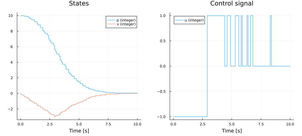
When plotting the solution, we see that the control signal indeed only takes integer values between mpc1.
plot!(plt[1], t, [sig(ssys.p1) sig(ssys.v1)]; seriestype = :steppre, linestyle = :dash, label = ["p (real)" "v (real)"])
plot!(plt[2], t, sig(ssys.u1); seriestype = :steppre, linestyle = :dash, label = "u (real)")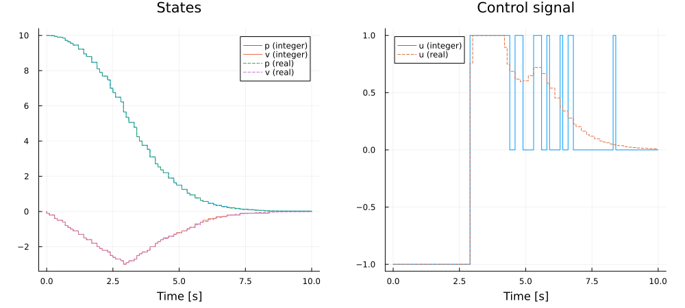
The state trajectories are almost identical (the system has strong low-pass character), but the control signal is much smoother when we allow the control input to take any real value.
Speed up computation
For some problems, computations can be sped up significantly by relaxing the integer constraints applied to control inputs towards the end of the optimization horizon. This possibility applies if
The control input corresponds to a real value and not, e.g., a mode of operation.
The system dynamics is of low-pass character.
As an example, take the temperature control of a room, with a heating element that can be either on or off as input. The binary constraint on the control input is in this case a technical limitation of the actuator, but an actuator supplying 50% of the heating power could just as well have been used. The plant is also of low-pass character, temperature variations are smoothed out due to the thermal inertia of the building. If we are solving this MPC problem with an MPC horizon of
We do this by specifying the integer horizon using the parameter Nc_binary, and the third loop of the model, with mpc3, shows the solution to the double integrator from above when
build_linear_mpc(A = [[1.0, 0.1], [0.0, 1.0]], B = [[0.0, 0.0], [0.1, -0.1]], Np = 10, Q1 = [1.0, 1.0], Q2 = [[0.100001, -0.1], [-0.1, 0.100001]], Qf = [10.0, 10.0], umin = [0.0, 0.0], umax = [1.0, 1.0], binary_controls = [1, 2], Nc_binary = 2, reference_tracking = false)plot!(plt[1], t, [sig(ssys.p3) sig(ssys.v3)]; seriestype = :steppre, linestyle = :dot, label = ["p (N_int = 2)" "v (N_int = 2)"])
plot!(plt[2], t, sig(ssys.u3); seriestype = :steppre, linestyle = :dot, label = "u (N_int = 2)")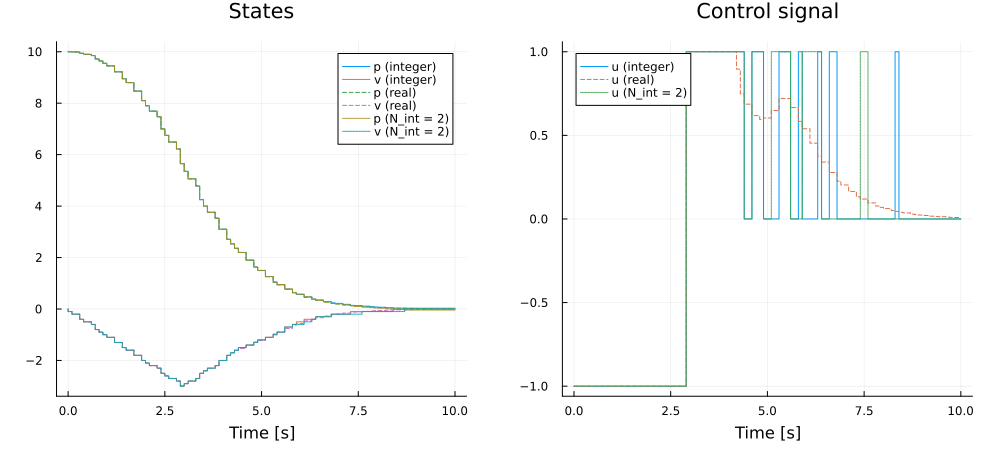
The state trajectory in this case is almost identical to the one obtained when all mpc_controllers lists the controllers of the model, and mpc_solve_time reports the cumulative time a controller has spent solving, so the difference around a simulation is the total solve time of each controller over the 100 samples, in seconds:
controllers = mpc_controllers(model)
solve_time(c) = mpc_solve_time(something(c.bundle, c.step))
t0 = solve_time.(controllers)
solve(prob)
[only(c.path) => solve_time(c) - t for (c, t) in zip(controllers, t0)]
3-element Vector{Pair{Symbol, Float64}}:
:mpc1 => 0.0005407081916928291
:mpc2 => 47.73866944434121
:mpc3 => 0.16980075370520353The intuition behind why this works is that the control decisions "far into the future" do not have a very large impact on what the first control input in the optimized trajectory should be, but the evolution of the state far into the future may still be important for constraint satisfaction, thus necessitating a long MPC horizon. With a low-pass system, replacing the integer values in the end of the control-signal trajectory with their "average values" is thus a good approximation.
Closing remarks
We have seen how we can force some variables in an MPC problem to be integer valued, in this case, the control input was constrained to belong to the set