TUTORIAL

Acausal Modeling and Creating Components

In this tutorial, we will build a simple RLC circuit from scratch (no external libraries like ElectricalComponents), and solve it using Dyad.

To get started, create a new component library, as indicated on the Getting started page.

Connector

First, let's start with the connector. Modeling physical systems always starts by defining connectors. This is because connectors are used to represent the information exchanged by components that interact with each other.

An electrical connector carries voltage and current. The declaration below illustrates its physical interface. This tutorial uses Dyad's built-in Pin, which also supplies the electrical port icons; keep that built-in definition when following the examples.

connector Pin
  potential v::Voltage
  flow i::Current
end

In Dyad, a typical connector is defined by matching pairs of potential and flow variables.

A connector may also declare stream fields, for intensive quantities such as specific enthalpy that are carried along by the flow, path fields, for a quantity that is defined in exactly one place across a network of connectors, and input/output fields, for causal signals. These are described in Connectors in the syntax manual; the RLC circuit built here needs only potential and flow.

Dyad includes connectors and units for the primary engineering domains. You can use them directly without adding a component library dependency.

The `flow` variable is generally the time derivative of a conserved quantity.

• Current (time derivative of charge)

• Torque (time derivative of angular momentum)

• Force (time derivative of linear momentum)

• Mass flow rate (time derivative of stored mass)

The sign convention used in Dyad is that flow is always positive into a component. Without a symmetric convention like this, it would matter which way you oriented a resistor or capacitor (which do not have an inherent orientation). For components where orientation matters, the icon will indicate how the orientation aligns with behavior.

If a component doesn't store the conserved quantity, the sum of all flow variables across all connectors associated with that quantity should be zero.

The potential variables are the quantities that drive this flow, e.g., differences in pressure, temperature, position, voltage, etc.

The built in connectors in Dyad are shown in the table below along with their choices for potential and flow variables:

Connector	Domain	potential	flow
Pin	Electrical	v::Voltage	i::Current
HeatPort	Thermal	T::Temperature	Q_flow::HeatFlowRate
Flange	Translational	s::Position	f::Force
Spline	Rotational	phi::Angle	tau::Torque

The physical types used in this connector, Voltage and Current (in fact, all ISO standard units) are also built in to Dyad, as are all the ISO standard units.

Components

Components declare parameters, variables, connectors, and relations. Create dyad/rlc_parts.dyad for the component definitions developed below.

A resistor is simply a component with two pins that obeys Ohm's law:

In Dyad, we can define this as follows:

component Resistor
  p = Pin()
  n = Pin()
  variable v::Voltage
  variable i::Current
  # Resistance of this resistor
  parameter R::Resistance
relations
  v = p.v - n.v
  i = p.i
  p.i + n.i = 0
  # Ohm's Law
  v = i * R
end

Similarly, we could define a capacitor:

component Capacitor
  p = Pin()
  n = Pin()
  variable v::Voltage
  variable i::Current
  # Capacitance of this capacitor
  parameter C::Capacitance
relations
  v = p.v - n.v
  i = p.i
  p.i + n.i = 0
  C * der(v) = i
end

But let's avoid repeating ourselves - you can notice the structural similarity between the resistor and capacitor.

Partial components

In Dyad, we can define partial components. A partial component is a component that is not complete, but can be used to build a complete component.

OnePort shares the two pins, voltage difference, and current balance. Its port metadata selects the built-in positive and negative pin icons and places them on opposite edges, using the placement from ElectricalComponents' TwoPin interface. Derived components inherit these placements.

Copy this complete definition into rlc_parts.dyad; it includes the metadata omitted from the viewer's Code pane:

partial component OnePort
  p = Pin() {^p}
  n = Pin() {^n}
  variable v::Voltage
  variable i::Current
relations
  v = p.v - n.v
  i = p.i
  p.i + n.i = 0
metadata {
  "_links": {
    "p": {
      "Dyad": {
        "placement": {"icon": {"iconName": "pos", "x1": -50, "y1": 450, "x2": 50, "y2": 550}}
      }
    },
    "n": {
      "Dyad": {
        "placement": {"icon": {"iconName": "neg", "x1": 950, "y1": 450, "x2": 1050, "y2": 550}}
      }
    }
  }
}
end

Then define the complete components by extending OnePort:

RLC Model

With all these components in place, we can build an RLC circuit model. In the dyad folder, create a new file named rlc.dyad and include the code below.

Analysis

Now that we have defined our component, we need a way to analyze it.

This is where the Dyad concept of an analysis comes in. Analyses are quite powerful. They not only provide out of the box workflows for doing things like performing a transient analysis or linearizing the equations of a system, they are extensible, i.e., users can create their own analyses. These new analyses (just like the ones built in ones) are written in Julia and have access to the fully symbolic problem statement.

For now, let's investigate the simplest case, a transient analysis. This is a simulation of the component over a given time span.

analysis SimRLC
  extends TransientAnalysis(stop=10, abstol=1m, reltol=1m)
  model = RLC()
end

Simulating

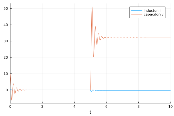
Save the model and analysis files, then click the Run Analysis play button beside SimRLC in the Analyses sidebar. The simulation opens a result plot and makes its result available as solution in the Julia REPL. To plot that result again from the REPL, run:

using Plots
plot(solution)