LIBRARY

Math.Tests.Ln
Computes the natural logarithm of constant and time-varying inputs.
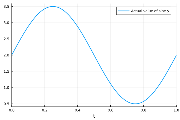
Connects a constant source with value e to a Ln block and verifies that ln(e) = 1. A second Ln block is driven by a sine wave (offset 2, amplitude 1.5) that stays strictly positive (0.5..3.5) as required by the logarithm domain while varying over time.
Usage
BlockComponents.Math.Tests.Ln()
Behavior
Source
dyad
"""
Computes the natural logarithm of constant and time-varying inputs.

Connects a constant source with value e to a Ln block and verifies that
ln(e) = 1. A second Ln block is driven by a sine wave (offset 2,
amplitude 1.5) that stays strictly positive (0.5..3.5) as required by the
logarithm domain while varying over time.
"""
test component Ln
  "Constant source providing the input value e"
  c1 = BlockComponents.Sources.Constant(k = 2.718281828459045) {
    "Dyad": {
      "placement": {
        "diagram": {"iconName": "default", "x1": 20, "y1": 10, "x2": 120, "y2": 110, "rot": 0}
      },
      "tags": []
    }
  }
  "Sine source kept strictly positive for the log domain"
  sine = BlockComponents.Sources.Sine(amplitude = 1.5, frequency = 1, offset = 2) {
    "Dyad": {
      "placement": {
        "diagram": {"iconName": "default", "x1": 20, "y1": 140, "x2": 120, "y2": 240, "rot": 0}
      },
      "tags": []
    }
  }
  "Ln block under test"
  ln_block = BlockComponents.Math.Ln() {
    "Dyad": {
      "placement": {
        "diagram": {"iconName": "default", "x1": 190, "y1": 10, "x2": 290, "y2": 110, "rot": 0}
      },
      "tags": []
    }
  }
  "Second Ln block driven by the sine source"
  ln_block_2 = BlockComponents.Math.Ln() {
    "Dyad": {
      "placement": {
        "diagram": {"iconName": "default", "x1": 200, "y1": 140, "x2": 300, "y2": 240, "rot": 0}
      },
      "tags": []
    }
  }
relations
  connect(c1.y, ln_block.u) {"Dyad": {"edges": [{"S": 1, "M": [], "E": 2}], "renderStyle": "standard"}}
  connect(sine.y, ln_block_2.u) {"Dyad": {"edges": [{"S": 1, "M": [], "E": 2}], "renderStyle": "standard"}}
metadata {
  "Dyad": {
    "icons": {"default": "dyad://BlockComponents/Example.svg"},
    "tests": {
      "case1": {"stop": 1, "expect": {"signals": ["ln_block.y", "ln_block_2.y", "sine.y"]}}
    }
  }
}
end
Flattened Source
dyad
"""
Computes the natural logarithm of constant and time-varying inputs.

Connects a constant source with value e to a Ln block and verifies that
ln(e) = 1. A second Ln block is driven by a sine wave (offset 2,
amplitude 1.5) that stays strictly positive (0.5..3.5) as required by the
logarithm domain while varying over time.
"""
test component Ln
  "Constant source providing the input value e"
  c1 = BlockComponents.Sources.Constant(k = 2.718281828459045) {
    "Dyad": {
      "placement": {
        "diagram": {"iconName": "default", "x1": 20, "y1": 10, "x2": 120, "y2": 110, "rot": 0}
      },
      "tags": []
    }
  }
  "Sine source kept strictly positive for the log domain"
  sine = BlockComponents.Sources.Sine(amplitude = 1.5, frequency = 1, offset = 2) {
    "Dyad": {
      "placement": {
        "diagram": {"iconName": "default", "x1": 20, "y1": 140, "x2": 120, "y2": 240, "rot": 0}
      },
      "tags": []
    }
  }
  "Ln block under test"
  ln_block = BlockComponents.Math.Ln() {
    "Dyad": {
      "placement": {
        "diagram": {"iconName": "default", "x1": 190, "y1": 10, "x2": 290, "y2": 110, "rot": 0}
      },
      "tags": []
    }
  }
  "Second Ln block driven by the sine source"
  ln_block_2 = BlockComponents.Math.Ln() {
    "Dyad": {
      "placement": {
        "diagram": {"iconName": "default", "x1": 200, "y1": 140, "x2": 300, "y2": 240, "rot": 0}
      },
      "tags": []
    }
  }
relations
  connect(c1.y, ln_block.u) {"Dyad": {"edges": [{"S": 1, "M": [], "E": 2}], "renderStyle": "standard"}}
  connect(sine.y, ln_block_2.u) {"Dyad": {"edges": [{"S": 1, "M": [], "E": 2}], "renderStyle": "standard"}}
metadata {
  "Dyad": {
    "icons": {"default": "dyad://BlockComponents/Example.svg"},
    "tests": {
      "case1": {"stop": 1, "expect": {"signals": ["ln_block.y", "ln_block_2.y", "sine.y"]}}
    }
  }
}
end
Test Cases
Test Case case1
julia
plt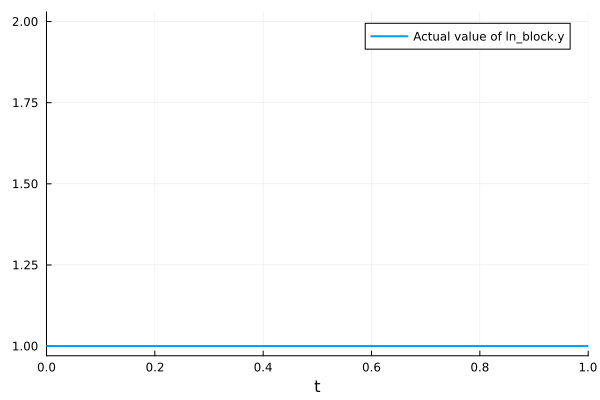
julia
plt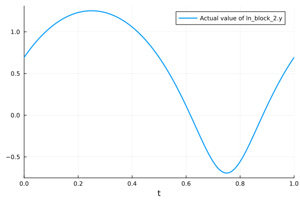
julia
plt