
Economic MPC for residential HVAC
This example will demonstrate the use of Model-Predictive Control (MPC) with an economic objective, i.e., we are solving a control problem where the cost function is economically motivated. The example we will consider is the control of indoor temperature in a residential building in southern Sweden, corresponding roughly to a single-family house.
The house in our example is equipped with a geothermal heat pump with a coefficient of performance (COP) of 4.9, i.e., for every kWh of electricity that is consumed by the heat pump, it delivers 4.9kWh of heat energy. The compressor in the heat pump can be run on 4 different power levels, each higher level consumes 1kW more than the previous, for a max power consumption of 4kW and thus a maximum heating capacity of 4.9*4 = 19.6kW.
The MPC controller will adjust the power level hourly, and it will make use of the following inputs
The current indoor temperature.
The outdoor temperature, available as a 24h forecast.
The spot price of electricity, available 24h into the future, obtained from the Nord Pool spot market.
In practice, weather forecasts are approximative, and the spot price for electricity is not always known 24h into the future, but for the purposes of this demonstration, these simplifying assumptions are made.[1]
We will make use of a very simple dynamical model that relates the indoor temperature to the power level of the heat pump, and the outdoor temperature. We use a week of temperature data obtained from SMHI and a week of electricity prices from the Nord Pool spot market for our simulation. The two series are available as HVAC_ELECTRICITY_PRICE and HVAC_OUTDOOR_TEMPERATURE in the module MPCComponents.Examples.HVAC.
using MPCComponents, Plots
using MPCComponents.Examples.HVAC: HVAC_ELECTRICITY_PRICE, HVAC_OUTDOOR_TEMPERATURE
using ModelingToolkit, SynchToolkit, OrdinaryDiffEqDefault
using ControlSystemsMTK, ControlSystemsBase
using Dates, Statistics, Printf

Ts  = 1   # Sample time hrs
heat_pump_power = 1  # kW per stage

electricity_price_kWh = HVAC_ELECTRICITY_PRICE # One week of hourly spot prices (SEK/100) at the Nord Pool energy market in area SE4
external_temperature  = HVAC_OUTDOOR_TEMPERATURE # One week of hourly temperatures in Hörby, Sweden

timevec = 0:Ts:length(electricity_price_kWh)-1
datevec = DateTime(Date("2023-02-24")):Dates.Hour(1):DateTime(Date("2023-03-02"), Time(23))

plot(datevec, [electricity_price_kWh/100 external_temperature], lab=["Electricity price SEK" "Temp °C"], title="A week in the end of February")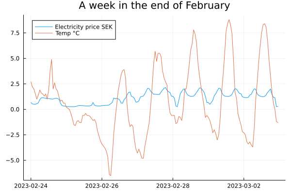
The figure above indicates that the price of electricity usually peaks during the morning and the evening, and is lowest during the night.
For the purposes of this tutorial, we will use a very simple dynamical model. The building is divided into 4 thermal masses, corresponding to walls, floor, circulating water and indoor air, and the time constants MPCComponents.Examples.HVAC.HVACPlant, whose definition we reproduce below. The heating gain input_gain includes the COP of the heat pump.
"""
Linear thermal model of a house heated by a heat pump through floor heating, the model of the
DyadControlSystems HVAC tutorial (https://help.juliahub.com/dyad/DyadControlSystems.jl/stable/examples/hvac/).
Four lumped temperatures — wall, indoor air, floor and circulating water — exchange heat with time
constants in hours; the heat pump's compressor power level `power` (kW, 0–4) heats the water and the
outdoor temperature `Text` acts on the wall. Time is in hours.

```math
\\begin{aligned}
\\dot T_{wall} &= (T_{ext} - T_{wall})/\\tau_{wall,ext} + (T_{int} - T_{wall})/\\tau_{wall,int} \\\\
\\dot T_{int} &= (T_{wall} - T_{int})/\\tau_{wall,int} + (T_{floor} - T_{int})/\\tau_{int,floor} \\\\
\\dot T_{floor} &= (T_{int} - T_{floor})/\\tau_{int,floor} + (T_{water} - T_{floor})/\\tau_{water,floor} \\\\
\\dot T_{water} &= (T_{floor} - T_{water})/\\tau_{water,floor} + k_{in}\\, power
\\end{aligned}
```

The output `y` is the indoor temperature. The model is linear, so `ControlSystemsMTK.named_ss(plant,
[plant.power, plant.Text], [plant.y])` gives its state-space matrices exactly; `HVACClosedLoop` takes
them (ZOH-discretized) as parameters for its MPC.
"""
component HVACPlant
  "Heat-pump compressor power level [kW]"
  power = RealInput() {^power}
  "Outdoor temperature [°C]"
  Text = RealInput() {^Text}
  "Indoor air temperature [°C]"
  y = RealOutput() {^y}
  "Wall–outdoor time constant [h]"
  parameter tau_wall_ext::Real = 48.0
  "Wall–indoor air time constant [h]"
  parameter tau_wall_int::Real = 18.0
  "Indoor air–floor time constant [h]"
  parameter tau_int_floor::Real = 3.6
  "Water–floor time constant [h]"
  parameter tau_water_floor::Real = 6.0
  "Heating gain of the compressor power [°C/(h kW)], COP 4.9 × 0.034"
  parameter input_gain::Real = 0.1666
  "Initial temperature of all four lumps [°C]"
  parameter T0::Real = 18.0
  "Wall temperature [°C]"
  variable Twall::Real
  "Indoor air temperature [°C]"
  variable Tint::Real
  "Floor temperature [°C]"
  variable Tfloor::Real
  "Circulating water temperature [°C]"
  variable Twater::Real
relations
  initial Twall = T0
  initial Tint = T0
  initial Tfloor = T0
  initial Twater = T0
  der(Twall) = (Text - Twall) / tau_wall_ext + (Tint - Twall) / tau_wall_int
  der(Tint) = (Twall - Tint) / tau_wall_int + (Tfloor - Tint) / tau_int_floor
  der(Tfloor) = (Tint - Tfloor) / tau_int_floor + (Twater - Tfloor) / tau_water_floor
  der(Twater) = (Tfloor - Twater) / tau_water_floor + input_gain * power
  y = Tint
metadata {
  "Dyad": {
    "icons": {"default": "dyad://MPCComponents/HVACPlant.svg"},
    "doc": {"behavior": false}
  },
  "_links": {
    "power": {
      "Dyad": {
        "placement": {
          "diagram": {"iconName": "default", "x1": -100, "y1": 350, "x2": 0, "y2": 450, "rot": 0}
        },
        "tags": []
      }
    },
    "Text": {
      "Dyad": {
        "placement": {
          "diagram": {"iconName": "default", "x1": -100, "y1": 550, "x2": 0, "y2": 650, "rot": 0}
        },
        "tags": []
      }
    },
    "y": {
      "Dyad": {
        "placement": {
          "diagram": {"iconName": "default", "x1": 1000, "y1": 450, "x2": 1100, "y2": 550, "rot": 0}
        },
        "tags": []
      }
    }
  }
}
end
We now linearize and discretize the model using a sampling time of 1 hour. Since the model is linear, the linearization is exact.
plant = complete(HVACPlant(; name = :plant))
G = named_ss(plant, [plant.power, plant.Text], [plant.y]) # Create a state space model
Gd = c2d(G, Ts)  # Discrete-time model

stepres = step(G, 7*24)
plot(stepres, title="One week step response", layout=(2,1), sp=[1 2], xlabel = "Time [hr]")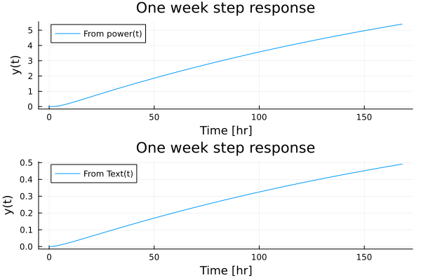
We are now ready to set up the MPC controller. The controller is the component LinearMPCController, and we start with some constants: the MPC optimization horizon Np of 24 hours, the initial state estimate x0 of the controller, and the setpoint Tref of the indoor temperature. In the closed-loop model below, these are the parameters
Np = 24
Tref = 20.0
x0 = [18.0, 18.0, 18.0, 18.0]
The state dimension of the model is 4, and the reference applies to the single controlled output, the indoor temperature, so we do not need to provide a reference for the other state components.
We then define the prediction model of the controller. It is the discrete-time model computed above, with the compressor power level as the control input and the outdoor temperature as a measured disturbance, and the output matrix selects the indoor temperature:
A  = Gd.A
B  = Gd.B[:, 1:1] # compressor power
Bd = Gd.B[:, 2:2] # outdoor temperature
C  = Gd.C
The controller receives the outdoor temperature as a forecast over the prediction horizon (disturbance_preview = true), which the component HVACForecast provides as a preview vector at every sample. The simulated plant receives the same outdoor temperature as a continuous signal from the component HVACWeather, held constant over each hour:
"""
Outdoor temperature of the tutorial week (hourly Hörby observations, held constant over each hour),
as a continuous signal: `y = hvac_outdoor_temperature(time)` with time in hours.
"""
component HVACWeather
  "Outdoor temperature [°C]"
  y = RealOutput() {^y}
relations
  y = hvac_outdoor_temperature(time)
metadata {
  "Dyad": {
    "icons": {"default": "dyad://MPCComponents/HVACWeather.svg"},
    "doc": {"behavior": false}
  },
  "_links": {
    "y": {
      "Dyad": {
        "placement": {
          "diagram": {"iconName": "default", "x1": 1000, "y1": 450, "x2": 1100, "y2": 550, "rot": 0}
        },
        "tags": []
      }
    }
  }
}
end
We also define cost functions for the MPC controller as well as some constraints. We assume a quadratic cost related to temperature deviations from the set point, increasing the penalty
The cost related to the input power is the monetary cost of electricity, here measured in SEK/100. LinearMPCController accepts a cost that is linear in the control, parameter_preview = true). We provide the hourly electricity price as this parameter, again through an HVACForecast, and Eu = [[1.0]] (the default Eu_gain = 1.0), so that the cost of the power level
and the corresponding parameters are
mpc = MPCComponents.LinearMPCController(final A = A, final B = B, final Bd = Bd, final C = C,
                                        final Np = Np,
                                        final Q1 = [Q1], final Q2 = [Q2], final Qf = [10.0 * Q1],
                                        final Eu = [[Eu_gain]],
                                        disturbance_preview = true, parameter_preview = true,
                                        ...)
with Q1 = 40 and Q2 = 0.001. The controller solves a convex quadratic program at every sample, so no initial guess of the solution is required.
Here, we include no constraints on the state vector, but including a lower bound on, either the indoor temperature or the maximum budget per day etc. could be considered. The power level is bounded to the range of the compressor:
umin = [0.0], umax = [4.0],The DyadControlSystems version of this tutorial assumes access to the full state for feedback. Here, the controller instead estimates the state from the measured indoor temperature, which is sampled through an A/D converter with a resolution of 12 bits (SampleWithADEffects), using an offset-free observer that also estimates a constant disturbance acting on the state (offset_free = StateDisturbance):
offset_free = MPCComponents.OffsetFreeMethod.StateDisturbance()Since the compressor has 4 discrete power levels, the DyadControlSystems version of this tutorial restricts the control input to integer values and solves a mixed-integer nonlinear program at every sample. Here, the power level is treated as a continuous variable between 0 and 4, and the resulting quadratic program is solved by DAQP through LinearMPC.jl. LinearMPCController also supports binary control inputs, with which integer-valued inputs can be encoded, see the tutorial MPC with binary or integer variables (MINLP).
We now package everything into a closed-loop model and simulate it. The electricity price and the outdoor temperature forecasts are generated by HVACForecast components from MPCComponents.Examples.HVAC, the controller samples the indoor temperature and the setpoint once every hour, and a zero-order hold applies the power level to the plant. The variables Tint, power and electricity_price make the signals of interest available for plotting.
"""
Economic MPC of the tutorial house: `HVACPlant` under a `LinearMPCController` that minimizes
`Q1 (Tint - Tref)^2 + price(t) * power` over a 24 h horizon with the hourly electricity price and outdoor
temperature forecasts (`HVACForecast`) as previewed generalized parameter and measured disturbance, the
power level bounded to 0–4 kW, and a `StateDisturbance` offset-free observer estimating the plant state
from the sampled indoor temperature. The compressor level is continuous here (the tutorial restricts it
to integers); a terminal weight `10 Q1` on the indoor temperature and a small `Q2` regularization complete
the quadratic cost.

The controller's model matrices `A`, `B` (power), `Bd` (outdoor temperature) and `C` (indoor temperature)
are parameters: obtain them from the plant with `ControlSystemsMTK.named_ss` and `c2d`. Analysis points
`u_ap`, `d_ap` and `y_ap` sit on the plant's inputs and output.
"""
example component HVACClosedLoop
  plant = HVACPlant() {^plant}
  weather = HVACWeather() {^weather}
  clock = DiscreteComponents.PeriodicClock(dt = 1.0) {^clock}
  reference = BlockComponents.Sources.Constant(k = Tref) {^reference}
  "Samples the setpoint"
  sample_r = DiscreteComponents.Sampler() {^sample_r}
  "Electricity price forecast over the horizon"
  price = MPCComponents.Examples.HVAC.HVACForecast(signal = MPCComponents.Examples.HVAC.HVACSignal.ElectricityPrice(), final Np = Np) {^price}
  "Outdoor temperature forecast over the horizon"
  forecast = MPCComponents.Examples.HVAC.HVACForecast(signal = MPCComponents.Examples.HVAC.HVACSignal.OutdoorTemperature(), final Np = Np) {^forecast}
  mpc = MPCComponents.LinearMPCController(final A = A, final B = B, final Bd = Bd, final C = C, final Np = Np, final Q1 = [Q1], final Q2 = [Q2], final Qf = [10.0 * Q1], final Eu = [[Eu_gain]], umin = [0.0], umax = [4.0], disturbance_preview = true, parameter_preview = true, offset_free = MPCComponents.OffsetFreeMethod.StateDisturbance(), x0 = [18.0, 18.0, 18.0, 18.0]) {^mpc}
  hold = DiscreteComponents.ZeroOrderHold() {^hold}
  samplewithadeffects = DiscreteComponents.SampleWithADEffects(y_min = -30, y_max = 50, bits = 12) {^samplewithadeffects}
  "Discrete-time state matrix of the plant (4 × 4), sample time 1 h"
  structural parameter A::Real[:, :]
  "Discrete-time input matrix of the compressor power (4 × 1)"
  structural parameter B::Real[:, :]
  "Discrete-time input matrix of the outdoor temperature (4 × 1)"
  structural parameter Bd::Real[:, :]
  "Output matrix selecting the indoor temperature (1 × 4)"
  structural parameter C::Real[:, :]
  "Prediction horizon [h]"
  structural parameter Np::Integer = 24
  "Weight on the squared indoor-temperature deviation"
  structural parameter Q1::Real = 40.0
  "Small regularization weight on the squared compressor power"
  structural parameter Q2::Real = 0.001
  "Gain of the electricity price in the cost of the controller; 0 removes the economic term"
  structural parameter Eu_gain::Real = 1.0
  "Indoor temperature setpoint [°C]"
  parameter Tref::Real = 20.0
  "Indoor temperature [°C]"
  variable Tint::Real
  "Compressor power level applied to the plant [kW]"
  variable power::Real
  "Electricity price [SEK/100 per kWh]"
  variable electricity_price::Real
relations
  Tint = plant.y
  power = hold.y
  electricity_price = hvac_electricity_price(time)
  connect(weather.y, plant.Text) {^id11}
  d_ap: analysis_point(weather.y, plant.Text)
  connect(hold.y, plant.power) {^id12}
  u_ap: analysis_point(hold.y, plant.power)
  y_ap: analysis_point(plant.y, samplewithadeffects.u)
  connect(clock.y, mpc.y[1], samplewithadeffects.y) {^id13}
  connect(reference.y, sample_r.u) {^id14}
  connect(sample_r.y, mpc.r[1]) {^id15}
  connect(forecast.y, mpc.d) {^id16}
  connect(price.y, mpc.p) {^id17}
  connect(mpc.u[1], hold.u) {^id18}
  connect(samplewithadeffects.u, plant.y) {^id19}
metadata {
  "Dyad": {
    "icons": {"default": "dyad://MPCComponents/HVACClosedLoop.svg"},
    "doc": {"behavior": false}
  },
  "_links": {
    "plant": {
      "Dyad": {
        "placement": {
          "diagram": {"iconName": "default", "x1": 700, "y1": 400, "x2": 800, "y2": 500, "rot": 0}
        },
        "tags": []
      }
    },
    "weather": {
      "Dyad": {"placement": {"diagram": {"x1": 500, "y1": 520, "x2": 600, "y2": 620}}}
    },
    "clock": {
      "Dyad": {"placement": {"diagram": {"x1": 470, "y1": 820, "x2": 530, "y2": 880}}}
    },
    "reference": {
      "Dyad": {"placement": {"diagram": {"x1": 20, "y1": 240, "x2": 120, "y2": 340}}}
    },
    "sample_r": {
      "Dyad": {"placement": {"diagram": {"x1": 150, "y1": 240, "x2": 250, "y2": 340}}}
    },
    "price": {
      "Dyad": {"placement": {"diagram": {"x1": 150, "y1": 370, "x2": 250, "y2": 470}}}
    },
    "forecast": {
      "Dyad": {"placement": {"diagram": {"x1": 150, "y1": 510, "x2": 250, "y2": 610}}}
    },
    "mpc": {
      "Dyad": {"placement": {"diagram": {"x1": 340, "y1": 390, "x2": 440, "y2": 490}}}
    },
    "hold": {
      "Dyad": {"placement": {"diagram": {"x1": 500, "y1": 390, "x2": 600, "y2": 490}}}
    },
    "samplewithadeffects": {
      "Dyad": {"placement": {"diagram": {"x1": 600, "x2": 500, "y1": 690, "y2": 790}}}
    },
    "id11": {
      "Dyad": {
        "edges": [{"S": 1, "M": [{"x": 650, "y": 570}, {"x": 650, "y": 460}], "E": 2}],
        "path": {}
      }
    },
    "id12": {"Dyad": {"edges": [{"S": 1, "M": [], "E": 2}], "path": {}}},
    "id13": {
      "Dyad": {
        "edges": [
          {"S": 1, "M": [{"x": 400, "y": 850}], "E": -1},
          {"S": -1, "M": [{"x": 310, "y": 740}, {"x": 310, "y": 474}], "E": 2},
          {"S": 3, "M": [], "E": -1}
        ],
        "junctions": [{"x": 400, "y": 740}],
        "path": {}
      }
    },
    "id14": {"Dyad": {"edges": [{"S": 1, "M": [], "E": 2}], "path": {}}},
    "id15": {
      "Dyad": {
        "edges": [{"S": 1, "M": [{"x": 290, "y": 290}, {"x": 290, "y": 402}], "E": 2}],
        "path": {}
      }
    },
    "id16": {
      "Dyad": {
        "edges": [{"S": 1, "M": [{"x": 290, "y": 560}, {"x": 290, "y": 453}], "E": 2}],
        "path": {}
      }
    },
    "id17": {
      "Dyad": {
        "edges": [{"S": 1, "M": [{"x": 280, "y": 420}, {"x": 280, "y": 425}], "E": 2}],
        "path": {}
      }
    },
    "id18": {
      "Dyad": {
        "edges": [{"S": 1, "M": [{"x": 480, "y": 428}, {"x": 480, "y": 440}], "E": 2}],
        "path": {}
      }
    },
    "id19": {
      "Dyad": {
        "edges": [{"S": 1, "M": [{"x": 840, "y": 740}, {"x": 840, "y": 450}], "E": 2}],
        "path": {}
      }
    }
  }
}
end
The matrices of the prediction model are structural parameters of the closed-loop model, which forwards them to the controller. The 24h forecasts require data up to the last hour of the week, so the closed loop is simulated for the first 143 hours.
@named model = HVACClosedLoop(; A, B, Bd, C)
ssys = mtkcompile(model; additional_passes = [SynchToolkit.compile_lustre])
prob = ODEProblem(ssys, [], (0.0, 143.0))
sol = solve(prob)
┌ Warning: Tracking with a direct penalty on the control (Q2) leaves a steady-state error on a plant with a finite static gain: u' Q2 u is minimized at u = 0, but holding the output at the reference needs a nonzero input. Leave Q2 empty (its default is zero) and penalize the control rate instead (Q3), which costs nothing at steady state. Q3 replaces Q2, not offset_free — a disturbance still needs an offset-free observer. Note that Q12 reintroduces the error for the same reason Q2 does.
└ @ LinearMPCRuntime ~/.julia/packages/MPCComponents/YhsiX/lib/LinearMPCRuntime/src/linear_mpc.jl:191For comparison, we solve the same problem also without the economic cost-function term, i.e., with a purely comfort-based cost. We obtain this controller by setting the structural parameter Eu_gain, which scales the gain Eu of the electricity price in the cost of the controller mpc, to zero:
## Non-economic MPC
@named model2 = HVACClosedLoop(; A, B, Bd, C, Eu_gain = 0.0)
ssys2 = mtkcompile(model2; additional_passes = [SynchToolkit.compile_lustre])
prob2 = ODEProblem(ssys2, [], (0.0, 143.0))
sol2 = solve(prob2)
┌ Warning: Tracking with a direct penalty on the control (Q2) leaves a steady-state error on a plant with a finite static gain: u' Q2 u is minimized at u = 0, but holding the output at the reference needs a nonzero input. Leave Q2 empty (its default is zero) and penalize the control rate instead (Q3), which costs nothing at steady state. Q3 replaces Q2, not offset_free — a disturbance still needs an offset-free observer. Note that Q12 reintroduces the error for the same reason Q2 does.
└ @ LinearMPCRuntime ~/.julia/packages/MPCComponents/YhsiX/lib/LinearMPCRuntime/src/linear_mpc.jl:191To visualize the result, we plot both solutions together. The power level applied during hour
xticks = 0:24:7*24
tk = 0:Ts:142
Tref = sol.ps[ssys.Tref]

temp  = sol(tk, idxs = ssys.Tint).u
temp2 = sol2(tk, idxs = ssys2.Tint).u
power  = sol(tk .+ Ts/2, idxs = ssys.power).u
power2 = sol2(tk .+ Ts/2, idxs = ssys2.power).u

total_cost  = sum(electricity_price_kWh[1:length(power)] .* power .* heat_pump_power .* Ts) / 100
total_cost2 = sum(electricity_price_kWh[1:length(power2)] .* power2 .* heat_pump_power .* Ts) / 100

err  = sqrt(mean(abs2, temp .- Tref))
err2 = sqrt(mean(abs2, temp2 .- Tref))

@printf("Total savings with price-aware predictive control: %2.1f%%\n", 100(total_cost2-total_cost)/total_cost2)
@printf("RMS temp deviation predictive control: %2.1f°C\n", err2)
@printf("RMS temp deviation price-aware predictive control: %2.1f°C\n", err)

plot(tk, temp; lab=@sprintf("Internal temperature (economic), RMS: %2.1f°C", err), xticks, layout=(2, 1), sp=1, linewidth=2, size=(800, 800), legendfontsize=7)
plot!(tk, power; seriestype=:steppost, lab=@sprintf("Heatpump power level (economic), cost: %2.0f SEK", total_cost), xticks, sp=2, linewidth=2)
plot!(tk, temp2; lab=@sprintf("Internal temperature (comfort), RMS: %2.1f°C", err2), sp=1, linewidth=2)
plot!(tk, power2; seriestype=:steppost, lab=@sprintf("Heatpump power level (comfort), cost: %2.0f SEK", total_cost2), sp=2, linewidth=2, plot_title="Economic MPC for temperature control")
hline!([Tref], lab="Setpoint", sp=1, color=1, linestyle=:dash)
plot!(timevec, external_temperature, lab="External temperature", sp=1, seriestype=:steppost, ylabel = "Temperature [°C]", xlabel = "Time [h]", margin=5Plots.mm)
plot!(timevec, electricity_price_kWh ./ 100, lab="Electricity price [SEK]", sp=2, seriestype=:steppost, xlabel = "Time [h]")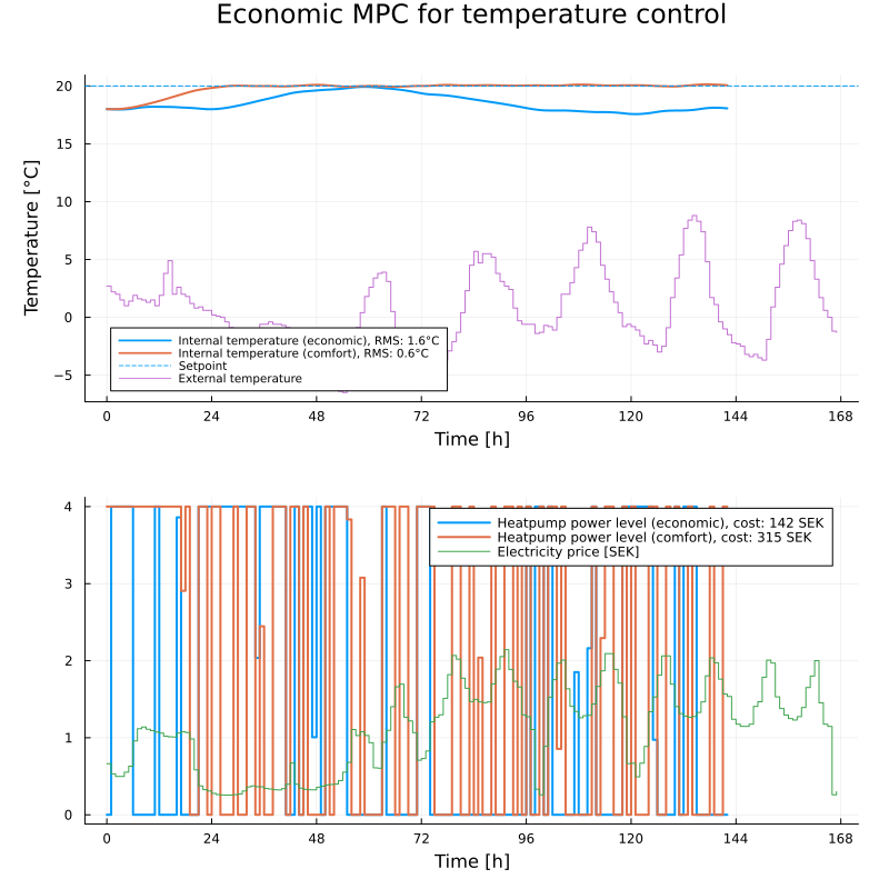
The figure indicates that the economic MPC controller uses more power at night when the electricity is cheap. It usually uses a bit of power during the typical lunch-time dip in prices as well. The comfort controller is oblivious to the price of electricity and is thus choosing to control the temperature much tighter, but does so to a significantly higher price. The economic controller keeps the indoor temperature below the setpoint throughout the week. Although the power level is a continuous variable here, both controllers apply one of its bounds, 0 or 4, in most hours and frequently alternate between them from one hour to the next.
Concluding remarks
In this example, we have made use of an MPC controller with an economically motivated cost function to minimize the price of heating a residential home using a geothermal heat pump, while keeping the indoor temperature at a comfortable level. The MPC controller ran with a prediction horizon of 24hrs and made use of (in this case perfect) forecasts of the spot price of electricity and the outdoor temperature.
While the economically motivated cost function appeals to the end user, it is also beneficial from a system perspective. The reason for the typically much cheaper electricity price at night is the significantly lower demand for electricity at night. By allocating the night hours for heating residential buildings, the peak load on the power grid that otherwise appears in the morning and afternoon is reduced.
Simplifying assumptions
In order to simplify the exposition of the MPC problem with an economic objective, this example made numerous simplifying and unrealistic assumptions:
The model used is very simplistic, and the prediction model of the controller is the exact discretization of the simulated plant.
The compressor power level is treated as a continuous variable, whereas the compressor can only be run on 4 discrete power levels.
The price is assumed known 24hrs in advance at all times. In practice, the price is known between 11 and 35 hrs in advance.
The outside temperature is assumed to be known exactly 24 hrs in advance. In practice, forecasts are inaccurate.
No external disturbances such as solar irradiation are modeled or simulated.
The cost of running the compressor in the heat pump at full capacity is not modeled, neither is the cost associated with frequent starts and stops of the compressor.
In practice, heat pumps must control not only the temperature of the indoor air, but also consider things like the temperature of the feed water as well as the temperature of the cold circuit to avoid overloading the bore hole etc.
The efficiency of the bore hole may decrease if too much energy is extracted during a short time period, this effect was not modeled.
The terminal cost used was naive. This can be improved by using longer-term forecasts or seasonal averages.
This example did not account for occupancy. At times when the building is unoccupied, the temperature can be allowed to deviate much more from the setpoint, thus simultaneously increasing the effective "storage capacity" of the building and reducing the amount of energy required to meet the comfort goals.
In practice, one may make use of longer forecasts of both weather and spot prices. This is likely beneficial due to the very long thermal time constants of many buildings. Planned power plant maintenance and unusually cold weather drive up electricity prices, both of which can be forecasted with reasonable accuracy. Thermally inert buildings may leverage the inertia to reduce the power consumption during forecasted price peaks.
Before an economically motivated controller is deployed in practice, it is important to validate the model and the controller in a realistic setting.
Each day at 13:00, the spot price per hour for the following day is determined on the Nord Pool electricity market, the electricity price is thus available between 11 and 35hrs in advance at all times. ↩︎