
MPC control of a Continuously Stirred Tank Reactor (CSTR)
The DyadControlSystems version of this tutorial, which uses a different MPC implementation, is available as a webinar:
The Continuously Stirred Tank Reactor (CSTR) is a common model for a chemical reactor. The model is available as the component MPCComponents.Examples.CSTRPlant, whose definition, including the model equations, we reproduce below
"""
Continuously stirred tank reactor with reactions A → B → C and 2A → D, controlled by the feed `F` and
the cooling-jacket heat flow `Qdot`. States: concentrations of A and B, reactor temperature, jacket
temperature. Translated from `DyadControlSystems.ControlDemoSystems.cstr` (time in hours).
"""
component CSTRPlant
  "Feed"
  F = RealInput() {^F}
  "Heat flow to the cooling jacket"
  Qdot = RealInput() {^Qdot}
  "Concentration of A"
  Ca_out = RealOutput() {^Ca_out}
  "Concentration of B"
  Cb_out = RealOutput() {^Cb_out}
  "Reactor temperature"
  Tr_out = RealOutput() {^Tr_out}
  "Cooling-jacket temperature"
  Tk_out = RealOutput() {^Tk_out}
  parameter K0_ab::Real = 1.287e12
  parameter K0_bc::Real = 1.287e12
  parameter K0_ad::Real = 9.043e9
  parameter E_A_ab::Real = 9758.3
  parameter E_A_bc::Real = 9758.3
  parameter E_A_ad::Real = 8560.0
  parameter Hr_ab::Real = 4.2
  parameter Hr_bc::Real = -11.0
  parameter Hr_ad::Real = -41.85
  parameter Rou::Real = 0.9342
  parameter Cp::Real = 3.01
  parameter Cpk::Real = 2.0
  parameter Ar::Real = 0.215
  parameter Vr::Real = 10.0
  parameter mk::Real = 5.0
  parameter T_in::Real = 130.0
  parameter K_w::Real = 4032.0
  parameter C_A0::Real = 5.1
  parameter Ca0::Real = 0.8
  parameter Cb0::Real = 0.5
  parameter Tr0::Real = 134.14
  parameter Tk0::Real = 130.0
  variable Ca::Real
  variable Cb::Real
  variable Tr::Real
  variable Tk::Real
  variable K1::Real
  variable K2::Real
  variable K3::Real
relations
  initial Ca = Ca0
  initial Cb = Cb0
  initial Tr = Tr0
  initial Tk = Tk0
  K1 = K0_ab * exp(-E_A_ab / (Tr + 273.15))
  K2 = K0_bc * exp(-E_A_bc / (Tr + 273.15))
  K3 = K0_ad * exp(-E_A_ad / (Tr + 273.15))
  der(Ca) = F * (C_A0 - Ca) - K1 * Ca - K3 * Ca ^ 2
  der(Cb) = -F * Cb + K1 * Ca - K2 * Cb
  der(Tr) = (K1 * Ca * Hr_ab + K2 * Cb * Hr_bc + K3 * Ca ^ 2 * Hr_ad) / (-Rou * Cp) + F * (T_in - Tr) + K_w * Ar * (Tk - Tr) / (Rou * Cp * Vr)
  der(Tk) = (Qdot + K_w * Ar * (Tr - Tk)) / (mk * Cpk)
  Ca_out = Ca
  Cb_out = Cb
  Tr_out = Tr
  Tk_out = Tk
metadata {
  "Dyad": {
    "icons": {"default": "dyad://MPCComponents/CSTRPlant.svg"},
    "doc": {"behavior": false}
  },
  "_links": {
    "F": {
      "Dyad": {"placement": {"diagram": {"x1": -100, "x2": 0, "y1": 260, "y2": 360}}}
    },
    "Qdot": {
      "Dyad": {"placement": {"diagram": {"x1": -100, "x2": 0, "y1": 650, "y2": 750}}}
    },
    "Ca_out": {
      "Dyad": {"placement": {"diagram": {"x1": 1000, "x2": 1100, "y1": 90, "y2": 190}}}
    },
    "Cb_out": {
      "Dyad": {"placement": {"diagram": {"x1": 1000, "x2": 1100, "y1": 340, "y2": 440}}}
    },
    "Tr_out": {
      "Dyad": {"placement": {"diagram": {"x1": 1000, "x2": 1100, "y1": 550, "y2": 650}}}
    },
    "Tk_out": {
      "Dyad": {"placement": {"diagram": {"x1": 1000, "x2": 1100, "y1": 790, "y2": 890}}}
    }
  }
}
end
The state dimension of the system is 4, the system has 2 inputs and strongly nonlinear dynamics. In particular, if the reaction
A depiction of a CSTR is shown below, a motor is continuously stirring the reactor contents, so we may assume that the contents are well mixed and the whole tank has a homogeneous temperature and concentration distribution.

The variables available for us to manipulate are the feed F and Qdot of CSTRPlant.
The component CSTRPlant contains the parameters of the model as well as the initial state of the system, Ca0, Cb0, Tr0 and Tk0. The controller is the component ACADOSMPC, and we will go through its parameters in the following sections. The parameters below specify the prediction model, the sample time Ts (hours), which is also the period of the clock that triggers the controller, the reference, and the MPC prediction horizon Np:
periodicclock = DiscreteComponents.PeriodicClock(dt = 0.005)
ref = BlockComponents.Sources.Constant(k = 0.6)
mpc = MPCComponents.ACADOSMPC(dynamics = plant,
                              inputs = ["F", "Qdot"],
                              state_variables = ["Ca", "Cb", "Tr", "Tk"],
                              outputs = ["Cb"],
                              Ts = 0.005,
                              Np = 30,
                              ...)
The prediction model is the plant component itself, dynamics = plant, with the control inputs named by inputs and the state variables listed in state_variables, in the order in which the controller receives them on its input x. The reference r does not have to be of the same length as the state, it has one entry per controlled output. We select the single output Cb and thereby indicate that we only have a reference for one of the state components and do not care about the others.
For improved numerics, ACADOSMPC accepts scaling vectors x_scale and u_scale that indicate the typical magnitudes of the state components and inputs, in which case the solver operates on the scaled variables. This improves the conditioning of the optimization problem when the state components have very different magnitudes, which is the case for this system. The controller in this tutorial converges without scaling, and we therefore leave these parameters at their default values.
For simulation purposes, the plant is integrated in continuous time by an ODE solver, and the controller samples its state once every Ts. The prediction model of the controller is built from dynamics = plant when the controller is constructed, and every parameter of the plant is then substituted by its default value, i.e., the controller predicts with the nominal parameters.
Creating constraints
The system has a number of constraints on inputs and the state that the MPC controller must respect: the feed is limited to umin and umax bound the control inputs, while constrained names the constrained signals of the model and constrained_max gives their upper bounds:
umin = [5.0, -8500.0],
umax = [100.0, 0.0],
constrained = ["Tr", "Tk"],
constrained_max = [142.0, 140.0],
Here, we have simple bounds constraints on the state, but ACADOSMPC also accepts general linear constraints on states and inputs, and, through nl_constrained, any nonlinear function of the signals of the model.
The state constraints are soft by default (state_bounds_soft = true), with a quadratic penalty on the constraint violation weighted by soft_weight. We use soft constraints for the temperatures to ensure that the optimizer handles constraint violations well. The input constraints are hard, since these can always be satisfied.
ACADOSMPC also allows for separate constraints on the terminal state terminal_constrained, terminal_constrained_min and terminal_constrained_max), making it efficient to implement simple terminal-set constraints.
Creating an objective
The control objective is to regulate the concentration of reactant ACADOSMPC minimizes the objective
where Q1, and do not penalize the control signal itself, Q2 = 0. The weights are matrices, and diagonal constructs a diagonal matrix from a vector.
We may also penalize the control-signal derivative (difference) by setting penalize_increments = true. The effect of this is that we penalize Q3. The prediction model is then augmented with the control signal as a state, and the control rate becomes the decision variable of the optimization problem. For improved convergence properties, the objective also includes a terminal cost, causing the optimizer to work hard to find a trajectory that ends up in the desired state. The terminal weight Qf defaults to Q1, so we do not specify it here. (We could also force the optimizer to end up in a terminal set, for this, we would have used the terminal constraints mentioned above.)
outputs = ["Cb"],
Q1 = diagonal([1.0]),
Q2 = diagonal([0.0, 0.0]),
penalize_increments = true,
Q3 = diagonal([5e-6, 2.5e-9]),
Creating an initial guess
The solver requires an initial guess for the optimal solution from the starting state. At the first sample, ACADOSMPC initializes the predicted trajectories with the measured state (or with x_guess when it is given) and with the control u_guess, which is also the control from which the first increment
u_guess = [10.0, -1000.0],At every subsequent sample, the solver starts from the solution of the previous sample, shifted by one step (warm_start).
Observer and solver
The MPC framework requires the specification of an observer that is responsible for feeding (an estimate of) the state of the system into the optimization part of the MPC controller. In this example, the four Sampler components sample the state of the plant directly, i.e., the controller does not rely on measurements, rather, it knows the state of the system from the simulation model. An observer such as UKFObserver may be connected between the plant and the controller input x instead.
The optimization problems are solved by acados using sequential quadratic programming (nlp_solver = SQP, the default), where each quadratic subproblem is solved by HPIPM. acados uses the Gauss-Newton approximation of the Hessian of the least-squares objective.
The infinite-dimensional continuous-time problem is transcribed to a finite-dimensional discrete-time problem by multiple shooting: acados integrates the prediction model over each of the Np shooting intervals. In this example, we use an implicit Runge-Kutta integrator (IRK) with 3 stages, whose stages are the Gauss-Legendre collocation points (the default collocation), a method suitable for stiff dynamics.
integrator = MPCComponents.ACADOSIntegrator.IRK(),
integrator_stages = 3,
Creating the closed-loop model
We are now ready to create the closed-loop model. The model below connects the plant and the controller configured above: the PeriodicClock with period Ts determines the sample instants, the samplers s convert the continuous-time state of the plant into the discrete-time controller input x, the sampler sr samples the reference, and the zero-order holds zoh hold the controls between samples. The variables Cb, Tr, Tk, F, Qdot and flag make the signals of interest available for plotting, flag being the acados status of each solve (0 indicates success).
"""
CSTR concentration control with `ACADOSMPC`, translated from the DyadControlSystems CSTR tutorial.
"""
example component CSTRMPCExample
  periodicclock = DiscreteComponents.PeriodicClock(dt = 0.005) {^periodicclock}
  plant = CSTRPlant() {^plant}
  "Samplers of the four state variables"
  s = [DiscreteComponents.Sampler() for i in 1:4] {^s}
  sr = DiscreteComponents.Sampler() {^sr}
  "Holds of the feed and the heat flow"
  zoh = [DiscreteComponents.ZeroOrderHold() for i in 1:2] {^zoh}
  "Concentration reference for B"
  ref = BlockComponents.Sources.Constant(k = 0.6) {^ref}
  mpc = MPCComponents.ACADOSMPC(dynamics = plant, inputs = ["F", "Qdot"], state_variables = ["Ca", "Cb", "Tr", "Tk"], outputs = ["Cb"], Ts = 0.005, Np = 30, Q1 = diagonal([1.0]), Q2 = diagonal([0.0, 0.0]), penalize_increments = true, Q3 = diagonal([5e-6, 2.5e-9]), umin = [5.0, -8500.0], umax = [100.0, 0.0], constrained = ["Tr", "Tk"], constrained_max = [142.0, 140.0], integrator = MPCComponents.ACADOSIntegrator.IRK(), integrator_stages = 3, u_guess = [10.0, -1000.0]) {^mpc}
  "Concentration of B"
  variable Cb::Real
  "Reactor temperature"
  variable Tr::Real
  "Jacket temperature"
  variable Tk::Real
  "Feed"
  variable F::Real
  "Heat flow"
  variable Qdot::Real
  "acados status"
  variable flag::Real
relations
  Cb = plant.Cb
  Tr = plant.Tr
  Tk = plant.Tk
  F = mpc.u[1]
  Qdot = mpc.u[2]
  flag = mpc.exitflag
  connect(plant.Ca_out, s[1].u) {^id8}
  connect(plant.Cb_out, s[2].u) {^id9}
  connect(plant.Tr_out, s[3].u) {^id10}
  connect(plant.Tk_out, s[4].u) {^id11}
  connect(ref.y, sr.u) {^id12}
  connect(s[1].y, mpc.x[1], periodicclock.y) {^id13}
  for i in 2:4
    connect(s[i].y, mpc.x[i])
  end
  connect(sr.y, mpc.r[1]) {^id14}
  for i in 1:2
    connect(mpc.u[i], zoh[i].u)
  end
  connect(zoh[1].y, plant.F)
  connect(zoh[2].y, plant.Qdot)
metadata {
  "Dyad": {"doc": {"behavior": false}},
  "_links": {
    "periodicclock": {
      "Dyad": {"placement": {"diagram": {"x1": 470, "x2": 570, "y1": 480, "y2": 580}}}
    },
    "plant": {
      "Dyad": {"placement": {"diagram": {"x1": 720, "x2": 820, "y1": 270, "y2": 370}}}
    },
    "s": {
      "Dyad": {"placement": {"diagram": {"x1": 570, "x2": 470, "y1": 720, "y2": 820}}}
    },
    "sr": {
      "Dyad": {"placement": {"diagram": {"x1": 160, "x2": 260, "y1": 230, "y2": 330}}}
    },
    "zoh": {
      "Dyad": {"placement": {"diagram": {"x1": 474, "x2": 574, "y1": 274, "y2": 374}}}
    },
    "ref": {
      "Dyad": {"placement": {"diagram": {"x1": 10, "x2": 110, "y1": 230, "y2": 330}}}
    },
    "mpc": {
      "Dyad": {"placement": {"diagram": {"x1": 340, "x2": 440, "y1": 311, "y2": 411}}}
    },
    "id8": {
      "Dyad": {
        "edges": [{"S": 1, "M": [{"x": 940, "y": 284}, {"x": 940, "y": 770}], "E": 2}],
        "path": {}
      }
    },
    "id9": {
      "Dyad": {
        "edges": [{"S": 1, "M": [{"x": 900, "y": 309}, {"x": 900, "y": 770}], "E": 2}],
        "path": {}
      }
    },
    "id10": {
      "Dyad": {
        "edges": [{"S": 1, "M": [{"x": 860, "y": 330}, {"x": 860, "y": 770}], "E": 2}],
        "path": {}
      }
    },
    "id11": {"Dyad": {"edges": [{"S": 1, "M": [{"x": 825, "y": 770}], "E": 2}], "path": {}}},
    "id12": {"Dyad": {"edges": [{"S": 1, "M": [], "E": 2}], "path": {}}},
    "id13": {
      "Dyad": {
        "edges": [
          {"S": 1, "M": [{"x": 280, "y": 770}, {"x": 280, "y": 361}], "E": 2},
          {"S": 2, "M": [{"x": 335, "y": 530}], "E": 3}
        ],
        "path": {}
      }
    },
    "id14": {
      "Dyad": {
        "edges": [{"S": 1, "M": [{"x": 320, "y": 280}, {"x": 320, "y": 326}], "E": 2}],
        "path": {}
      }
    }
  }
}
end
We instantiate the model in Julia and compile it. Models that contain clocked (discrete-time) components, such as the controller, are compiled with the additional pass SynchToolkit.compile_lustre, which compiles the discrete-time partitions of the model.
@named model = CSTRMPCExample()
ssys = mtkcompile(model; additional_passes = [SynchToolkit.compile_lustre])
Run MPC controller
We may now simulate the closed-loop system over 50 sample intervals, i.e., 0.25 hours. The plant is simulated in continuous time by the ODE solver, while the controller predicts with the model it was built from, integrated by acados. The simulation model thus does not have to be the same as the prediction model, which we make use of in the next section.
prob = ODEProblem(ssys, [], (0.0, 0.25))
sol = solve(prob)
plot(sol, idxs = [ssys.plant.Ca, ssys.plant.Cb, ssys.plant.Tr, ssys.plant.Tk], layout = (3, 2), sp = [1 2 3 4], xlabel = "Time [hrs]", lab = "")
plot!(sol, idxs = [ssys.F, ssys.Qdot], sp = [5 6], xlabel = "Time [hrs]", lab = "")
hline!([sol.ps[ssys.ref.k]], sp = 2, l = (:green, :dash), lab = "Reference")
hline!([142.0 140.0], sp = [3 4], ls = :dash, lw = 1, color = :black, lab = "Upper bound")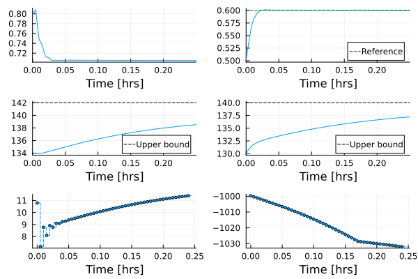
The result should indicate that the state
Enter uncertainty
What would happen if the plant model does not exactly match reality? We could simulate the effect of a model mismatch in one or several of the parameters by supplying a different parameter value for the plant when we create the ODEProblem; the controller keeps predicting with the nominal values it was built with. Below, we simulate that the actual activation energy for the reaction
E_A_ad = prob.ps[ssys.plant.E_A_ad] # nominal value
prob_u = ODEProblem(ssys, [ssys.plant.E_A_ad => 0.95E_A_ad], (0.0, 0.25))
sol_u = solve(prob_u)
plot(sol_u, idxs = [ssys.plant.Ca, ssys.plant.Cb, ssys.plant.Tr, ssys.plant.Tk], layout = (3, 2), sp = [1 2 3 4], xlabel = "Time [hrs]", lab = "")
plot!(sol_u, idxs = [ssys.F, ssys.Qdot], sp = [5 6], xlabel = "Time [hrs]", lab = "")
hline!([sol_u.ps[ssys.ref.k]], sp = 2, l = (:green, :dash), lab = "Reference")
hline!([142.0 140.0], sp = [3 4], ls = :dash, lw = 1, color = :black, lab = "Upper bound")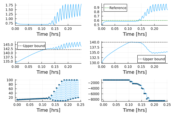
This time, both temperatures exceed the safe operating bounds, the reactor temperature by several degrees, and the state
Summary
This tutorial has demonstrated the use of constrained nonlinear MPC by means of the ACADOSMPC component on a highly nonlinear MIMO system, using an implicit Runge-Kutta integrator with Gauss-Legendre collocation points for the transcription.
using Test
@test sol(0.25, idxs = ssys.Cb) ≈ 0.6 atol = 1e-3
@test all(sol(0:0.005:0.25, idxs = ssys.flag) .== 0)
Test Passed