
Linear Analysis
Download as a Dyad projectLinearExample.zipOpen in Dyad Studio
The Linear Analysis computes the linearized dynamics of a model and provides a suite of frequency- and time-domain analysis tools. This is useful for understanding the small-signal behavior of a system, including stability, resonance, and transient response.
Method Overview
Linear analysis is performed by linearizing the provided model around an operating point. The resulting linear system can be analyzed using classical control theory tools, including:
Frequency response (Bode, Nyquist, root locus, and RGA plots)
Time response (step response, rise time, settling time, overshoot, etc.)
Modal analysis (damping report, pole-zero map)
Symbolic linearization
Set symbolic = true in DyadControlSystems.LinearAnalysis to inspect how a small model's dynamics depend on its parameters. This option, available in DyadControlSystems 2.4.2, adds a symbolic linearization alongside the numerical result. Its
For example, the mass-spring-damper equation
Choose a small, smooth model for this option:
Branching expressions such as
ifelse,max,min,clamp, and saturation blocks are unsupported. The motor example below uses a controller with limiters and demonstrates numerical linearization only.Differential-algebraic models require a symbolic linear solve without pivoting; results can be unreliable or fail for higher-index systems.
Expressions and computation costs grow rapidly with state dimension.
SymbolicPolesrequiresusing Nemoin the Julia session. Its closed-form root solver is limited to degree four after cancellation of trivial factors; this restriction does not apply to the other symbolic artifacts.
The symbolic result is a separate linearization: its state order and dimension may differ from the reduced numerical system. The analysis's t setting applies to the numerical result; symbolic expressions retain explicit time dependence.
For use directly from Julia, DyadControlSystems provides named_ss_symbolic, symbolic_charpoly, symbolic_poles, and symbolic_tf. After loading DyadControlSystems, enter ?named_ss_symbolic in the Julia REPL for the API and a worked example.
Example Definition
Since we are opening the loop at r (the reference speed input to the controller), we need to provide an initial condition for controller.u_s — otherwise, the linearization cannot determine its operating point value. We do this by extending the test model and adding initial controller.u_s = 0:
component DCMotorForLinearization
  extends DyadExampleComponents.TestDCMotorLoadControlled(w_motor = 0)
relations
  guess controller.u_s = 0
  guess controller.u_m = 0
  guess motor.R1.v = 0
  guess motor.emf.tau = 0
  guess motor.emf.rotor.tau = 0
  guess motor.emf.rotor.phi = 0
  guess motor.emf.p.i = 0
  guess motor.friction.phi_rel = 0
  guess load.phi = 0
  guess controller.proportional.y = 0
  guess controller.add_pid.y = 0
  guess controller.derivative.y = 0
end

analysis DCMotorLinearAnalysis
  extends DyadControlSystems.LinearAnalysis(
    outputs       = ["y"],
    inputs        = ["r"],
    loop_openings = ["r"],
    duration = 5.0
  )
  model = DCMotorForLinearization()
end
We set w_motor to zero so the controller does not saturate at the linearization point, and provide guess controller.u_s = 0 so the disconnected setpoint input has a defined operating point. We also provide numeric guesses for the algebraic motor variables and the controller's internal block outputs so that the linearization solver does not encounter cyclic guesses.
using DyadInterface: artifacts
asol = DCMotorLinearAnalysis()
artifacts(asol, :StepInfoPlot)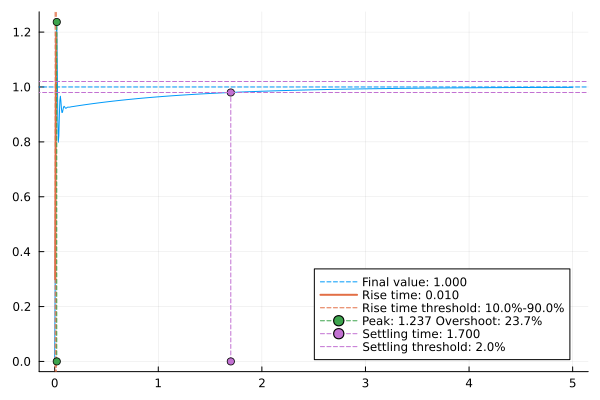
artifacts(asol, :BodePlot)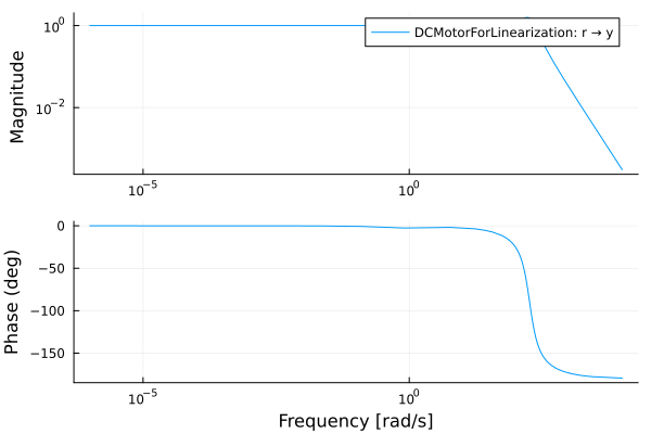
artifacts(asol, :DampReport)| Row | Pole | DampingRatio | Frequency_rad_s | Frequency_Hz | TimeConstant_s |
|---|---|---|---|---|---|
| Complex… | Float64 | Float64 | Float64 | Float64 | |
| 1 | -0.00010001+0.0im | 1.0 | 0.00010001 | 1.59171e-5 | 9999.0 |
| 2 | -0.834172+0.0im | 1.0 | 0.834172 | 0.132763 | 1.19879 |
| 3 | -55.3885+173.864im | 0.303543 | 182.473 | 29.0415 | 0.0180543 |
Analysis Arguments
The following arguments define a LinearAnalysis:
Required Arguments
model: The model to be analyzed.inputs::Vector{String}: Names of the input analysis pointsoutputs::Vector{String}: Names of the output analysis points
Optional Arguments
wl::Real = -1: Lower frequency bound for Bode plot (set to -1 for automatic selection).wu::Real = -1: Upper frequency bound for Bode plot (set to -1 for automatic selection).num_frequencies::Int = 3000: Number of frequency points.duration::Real = -1: Duration for the step response plot (set to -1 for automatic selection).loop_openings::Vector{String} = []: Analysis points where feedback loops are opened before linearization.t::Real = 0: Time at which to compute the numerical linearization.symbolic::Bool = false: Also compute the symbolic linearization.
Artifacts
A LinearAnalysis returns the following artifacts:
Standard Plots
BodePlot: Bode plot of the system.MarginPlot: Bode plot with gain margin and phase margin.StepResponse: Step response of the system.StepInfoPlot: Plot of step response characteristics.RootLocusPlot: Root locus plot of the system.PoleZeroMap: Pole-zero map of the system.NyquistPlot: Nyquist plot of the system.RGAPlot: Relative Gain Array (RGA) plot of the system.
Tables
DampReport: DataFrame with modal analysis (damping, frequency, time constant, etc.).StepInfo: DataFrame with step response characteristics.ObservabilityReport: DataFrame with observability information.
Symbolic Results
With symbolic = true, the result also provides:
| Artifact | Result |
|---|---|
SymbolicStateSpace | State-space system with symbolic |
SymbolicMatrices | Full symbolic Jacobians, including descriptor blocks for differential-algebraic models. |
CharacteristicPolynomial | Characteristic polynomial |
SymbolicPoles | Closed-form poles; requires Nemo and the degree limit described above. |
SymbolicTransferFunction | Transfer function |
For a result computed with symbolic = true, use artifacts(result, :SymbolicStateSpace) or another artifact name from the table. Derived expressions are computed when requested; only the poles require Nemo.