Trimming

Trimming, or determining an operating point, of a dynamic system, involves finding a state and input to the system dynamics that satisfy user-defined constraints. Trimming is commonly used as a first step in determining a point about which to linearize a nonlinear system.

A tutorial on trimming in the form of a webinar is available below

Trim vs Equilibrium Points:

A special case of trimming is finding an equilibrium point of a dynamic system. An equilibrium point is a feasible steady state of the dynamic system, i.e., a state at which all the derivatives are zero, $f(x, u, p, t) = 0$. Trimming can be applied to many dynamic system formalisms; this document will discuss ODE systems and DAE systems.

ODE Systems

Consider an ODE system $\dot x = f(x,u,p,t)$ where $x \in \mathbb{R}^n$ are the state variables, $u \in \mathbb{R}^m$ control input variables, $p$ are the parameters and $f:\mathbb{R}^{n} \times \mathbb{R}^{m} \mapsto \mathbb{R}^n$ is a potentially nonlinear function. An equilibrium point $(x_{eq}, u_{eq})$ is a solution to the set of nonlinear equations $f(x_{eq}, u_{eq}, p, t) = \mathbf{0}$. This point is generally not unique since the equation system has $n+m$ variables and $n$ equations.

Various methods may be used to determine the equilibrium point: For instance, one may use the a root-finding algorithm to solve the system of nonlinear equations above. In addition, a constrained-optimization problem may be formulated which in general is a nonconvex nonlinear program (NLP). Alternatively, an unconstrained optimization problem may be formulated by using a penalty function to dualize the constraints.

Trim points generalize the concept of equilibrium points: A user may want to impose additional hard or soft constraints (defined by equations or inequalities involving the states of the system). In addition, a user may specify certain derivatives to be non-zero. Unlike equilibrium points which may be determined using root-finding algorithms, it is usually necessary to formulate a constrained or unconstrained optimization problem to determine trim points as is done in the developed trim function.

Trimming Workflow:

1. The dynamic system here named sys is defined symbolically using the ModelingToolkit framework, thus sys is of type AbstractSystem. This system should not be simplified by the user by calling structural_simplify as this is done inside the trim function.

• Next the trim function is called. If the system is unbalanced, i.e., if the number of states exceeds the number of equations as a result of having certain control inputs, it is necessary to specify an array of control inputs and outputs using the inputs and outputs arguments.
• Optionally, to determine a trim point, the user may specify certain desired states, hard or soft inequality or equality constraints using the corresponding arguments. If none of these are specified, the function returns an equilibrium point.
• By default, the internals of the trim function involve formulating a constrained optimization problem. The user may want to specify tailored penalty multipliers or use the penalty function approach to dualize the contraints such that an unconstrained optimization problem is formulated instead. In either case, it is essential to specify an appropriate optimization solver.

Example: The nonlinear Research Civil Aircraft Model (RCAM)

The trim functionality is illustrated using the nonlinear Research Civil Aircraft Model (RCAM) developed by GARTEUR and using the derivations and errata presented by Prof. Christopher Lum. An open-source implementation of this model is also presented in PSim-RCAM.

Figure 1: Aircraft axes and control surfaces. Figure attained from Wikimedia Commons with CC by 4.0 license,

The RCAM model has the following 9 states:

• \[u, v, w\]

  : the translational velocity [m/s] in the body frame in the x, y and z-axes respectively,

• \[p, q, r\]

  : the rotational velocity [rad/s] in the body frame about the x (roll/bank), y (pitch) and z (yaw)-axes respectively,

• \[ϕ, θ, ψ\]

  : the rotation angles [rad] in the body frame about the x (roll/bank), y (pitch) and z (yaw)-axes respectively,

and the following 5 control inputs:

• \[u_A\]

  : the aileron angle [rad]

• \[u_T\]

  : the tail angle [rad]

• \[u_R\]

  : the rudder angle [rad]

• \[u_{E1}\]

  : the left engine/throttle position [rad]

• \[u_{E2}\]

  : the right engine/throttle position [rad]

The mechanistic model is defined symbolically as an ODESystem in ModelingToolkit using the 9-step procedure and parameters detailed in this lecture.

1.a. First, the parameters for the model are defined as follows:

using ModelingToolkit, OrdinaryDiffEq, ModelingToolkit.IfElse, JuliaSimControl
using LinearAlgebra:cross, inv
using Plots

# Define a dictionary of constants

rcam_constants = Dict(:m => 120000.0, :c̄ => 6.6, :lt => 24.8, :S => 260.0, :St => 64.0, :Xcg => 0.23 * 6.6,:Ycg => 0.0, :Zcg => 0.10 * 6.6, :Xac => 0.12 * 6.6, :Yac => 0.0, :Zac => 0.0, :Xapt1 => 0.0, :Yapt1 => -7.94, :Zapt1 => -1.9, :Xapt2 => 0.0, :Yapt2 => 7.94, :Zapt2 => -1.9, :g => 9.81, :depsda => 0.25, :α_L0 => deg2rad(-11.5), :n => 5.5, :a3 => -768.5, :a2 => 609.2, :a1 => -155.2, :a0 => 15.212, :α_switch => deg2rad(14.5), :ρ => 1.225)

Ib_mat =  [40.07          0.0         -2.0923
            0.0            64.0        0.0
            -2.0923        0.0         99.92]*rcam_constants[:m]

Ib = Ib_mat
invIb = inv(Ib_mat)

ps = @parameters(
        ρ             = rcam_constants[:ρ], [description="kg/m3 - air density"],
        m             = rcam_constants[:m], [description="kg - total mass"],
        c̄          = rcam_constants[:c̄], [description="m - mean aerodynamic chord"],
        lt            = rcam_constants[:lt], [description="m - tail AC distance to CG"],
        S             = rcam_constants[:S], [description="m2 - wing area"],
        St            = rcam_constants[:St], [description="m2 - tail area"],
        Xcg           = rcam_constants[:Xcg], [description="m - x pos of CG in Fm"],
        Ycg           = rcam_constants[:Ycg], [description="m - y pos of CG in Fm"],
        Zcg           = rcam_constants[:Zcg], [description="m - z pos of CG in Fm"],
        Xac           = rcam_constants[:Xac], [description="m - x pos of aerodynamic center in Fm"],
        Yac           = rcam_constants[:Yac], [description="m - y pos of aerodynamic center in Fm"],
        Zac           = rcam_constants[:Zac], [description="m - z pos of aerodynamic center in Fm"],
        Xapt1         = rcam_constants[:Xapt1], [description="m - x position of engine 1 in Fm"],
        Yapt1         = rcam_constants[:Yapt1], [description="m - y position of engine 1 in Fm"],
        Zapt1         = rcam_constants[:Zapt1], [description="m - z position of engine 1 in Fm"],
        Xapt2         = rcam_constants[:Xapt2], [description="m - x position of engine 2 in Fm"],
        Yapt2         = rcam_constants[:Yapt2], [description="m - y position of engine 2 in Fm"],
        Zapt2         = rcam_constants[:Zapt2], [description="m - z position of engine 2 in Fm"],
        g             = rcam_constants[:g], [description="m/s2 - gravity"],
        depsda        = rcam_constants[:depsda], [description="rad/rad - change in downwash wrt α"],
        α_L0      = rcam_constants[:α_L0], [description="rad - zero lift AOA"],
        n             = rcam_constants[:n], [description="adm - slope of linear ragion of lift slope"],
        a3            = rcam_constants[:a3], [description="adm - coeff of α^3"],
        a2            = rcam_constants[:a2], [description="adm -  - coeff of α^2"],
        a1            = rcam_constants[:a1], [description="adm -  - coeff of α^1"],
        a0            = rcam_constants[:a0], [description="adm -  - coeff of α^0"],
        α_switch  = rcam_constants[:α_switch], [description="rad - kink point of lift slope"]
    )

1.b. Next the 9 states and 5 control variables are defined:

@parameters t
D =  Differential(t)

# States
V_b = @variables(
    u(t), [description="translational velocity along x-axis [m/s]"],
    v(t), [description="translational velocity along y-axis [m/s]"],
    w(t), [description="translational velocity along z-axis [m/s]"]
    )

wbe_b = @variables(
    p(t), [description="rotational velocity about x-axis [rad/s]"],
    q(t), [description="rotational velocity about y-axis [rad/s]"],
    r(t), [description="rotational velocity about z-axis [rad/s]"]
    )

rot = @variables(
    ϕ(t), [description="rotation angle about x-axis/roll or bank angle [rad]"],
    θ(t), [description="rotation angle about y-axis/pitch angle [rad]"],
    ψ(t), [description="rotation angle about z-axis/yaw angle [rad]"]
    )

# Controls
U = @variables(
    uA(t), [description="aileron [rad]"],
    uT(t), [description="tail [rad]"],
    uR(t), [description="rudder [rad]"],
    uE_1(t), [description="throttle 1 [rad]"],
    uE_2(t), [description="throttle 2 [rad]"],
)

1.c. Next, the auxiliary variables and intermediate system of equations is defined:

# Auxiliary Variables to define model.

Auxiliary_vars = @variables Va(t) α(t) β(t) Q(t) CL_wb(t) ϵ(t) α_t(t) CL_t(t) CL(t) CD(t) CY(t) F1(t) F2(t)

@variables FA_s(t)[1:3] C_bs(t)[1:3,1:3] FA_b(t)[1:3] eta(t)[1:3] dCMdx(t)[1:3, 1:3] dCMdu(t)[1:3, 1:3] CMac_b(t)[1:3] MAac_b(t)[1:3] rcg_b(t)[1:3] rac_b(t)[1:3] MAcg_b(t)[1:3] FE1_b(t)[1:3] FE2_b(t)[1:3] FE_b(t)[1:3] mew1(t)[1:3] mew2(t)[1:3] MEcg1_b(t)[1:3] MEcg2_b(t)[1:3] MEcg_b(t)[1:3] g_b(t)[1:3] Fg_b(t)[1:3] F_b(t)[1:3] Mcg_b(t)[1:3] H_phi(t)[1:3,1:3]

# Scalarizing all the array variables.

FA_s = collect(FA_s)
C_bs = collect(C_bs)
FA_b = collect(FA_b)
eta = collect(eta)
dCMdx = collect(dCMdx)
dCMdu = collect(dCMdu)
CMac_b =  collect(CMac_b)
MAac_b = collect(MAac_b)
rcg_b = collect(rcg_b)
rac_b = collect(rac_b)
MAcg_b = collect(MAcg_b)
FE1_b = collect(FE1_b)
FE2_b = collect(FE2_b)
FE_b = collect(FE_b)
mew1 = collect(mew1)
mew2 = collect(mew2)
MEcg1_b = collect(MEcg1_b)
MEcg2_b = collect(MEcg2_b)
MEcg_b = collect(MEcg_b)
g_b = collect(g_b)
Fg_b = collect(Fg_b)
F_b = collect(F_b)
Mcg_b = collect(Mcg_b)
H_phi = collect(H_phi)

array_vars = vcat(vec(FA_s), vec(C_bs), vec(FA_b), vec(eta), vec(dCMdx), vec(dCMdu), vec(CMac_b), vec(MAac_b), vec(rcg_b), vec(rac_b), vec(MAcg_b), vec(FE1_b), vec(FE2_b), vec(FE_b), vec(mew1), vec(mew2), vec(MEcg1_b), vec(MEcg2_b), vec(MEcg_b), vec(g_b), vec(Fg_b), vec(F_b), vec(Mcg_b), vec(H_phi))

eqns =[
    # Step 1. Intermediate variables
    # Airspeed
    Va ~ sqrt(u^2 + v^2 + w^2)

    # α and β
    α ~ atan(w,u)
    β ~ asin(v/Va)

    # dynamic pressure
    Q ~ 0.5*ρ*Va^2


    # Step 2. Aerodynamic Force Coefficients
    # CL - wing + body
    #CL_wb ~  n*(α - α_L0)

    CL_wb ~ IfElse.ifelse(α <= α_switch, n*(α - α_L0), a3*α^3 + a2*α^2 + a1*α + a0)

    # CL thrust
    ϵ ~ depsda*(α - α_L0)
    α_t ~ α - ϵ + uT + 1.3*q*lt/Va
    CL_t ~ 3.1*(St/S) * α_t

    # Total CL
    CL ~ CL_wb + CL_t

    # Total CD
    CD ~ 0.13 + 0.07 * (n*α + 0.654)^2

    # Total CY
    CY ~ -1.6*β + 0.24*uR


    # Step 3. Dimensional Aerodynamic Forces
    # Forces in F_s
    FA_s .~ [-CD * Q * S
                CY * Q * S
                -CL * Q * S]


    # rotate forces to body axis (F_b)
    vec(C_bs .~ [cos(α)      0.0      -sin(α)
                    0.0             1.0      0.0
                    sin(α)      0.0      cos(α)])


    FA_b .~ C_bs*FA_s

    # Step 4. Aerodynamic moment coefficients about AC
    # moments in F_b
    eta .~ [ -1.4 * β
                -0.59 - (3.1 * (St * lt) / (S * c̄)) * (α - ϵ)
            (1 - α * (180 / (15 * π))) * β
    ]


    vec(dCMdx .~ (c̄ / Va)*        [-11.0              0.0                           5.0
                                        0.0   (-4.03 * (St * lt^2) / (S * c̄^2))        0.0
                                        1.7                 0.0                          -11.5])


    vec(dCMdu .~ [-0.6                   0.0                 0.22
                    0.0   (-3.1 * (St * lt) / (S * c̄))      0.0
                    0.0                    0.0                -0.63])

    # CM about AC in Fb
    CMac_b .~ eta + dCMdx*wbe_b + dCMdu*[uA
                                        uT
                                        uR]

    # Step 5. Aerodynamic moment about AC
    # normalize to aerodynamic moment
    MAac_b .~ CMac_b * Q * S * c̄

    # Step 6. Aerodynamic moment about CG
    rcg_b .~    [Xcg
                Ycg
                Zcg]

    rac_b .~ [Xac
            Yac
            Zac]

    MAcg_b .~ MAac_b + cross(FA_b, rcg_b - rac_b)

    # Step 7. Engine force and moment
    # thrust
    F1 ~ uE_1 * m * g
    F2 ~ uE_2 * m * g

    # thrust vectors (assuming aligned with x axis)
    FE1_b .~ [F1
                0
                0]

    FE2_b .~ [F2
                0
                0]

    FE_b .~ FE1_b + FE2_b

    # engine moments
    mew1 .~  [Xcg - Xapt1
            Yapt1 - Ycg
            Zcg - Zapt1]

    mew2 .~ [ Xcg - Xapt2
            Yapt2 - Ycg
            Zcg - Zapt2]

    MEcg1_b .~ cross(mew1, FE1_b)
    MEcg2_b .~ cross(mew2, FE2_b)

    MEcg_b .~ MEcg1_b + MEcg2_b

    # Step 8. Gravity effects
    g_b .~ [-g * sin(θ)
            g * cos(θ) * sin(ϕ)
            g * cos(θ) * cos(ϕ)]

    Fg_b .~ m * g_b

    # Step 9: State derivatives

    # form F_b and calculate u, v, w dot
    F_b .~ Fg_b + FE_b + FA_b

    D.(V_b) .~ (1 / m)*F_b - cross(wbe_b, V_b)

    # form Mcg_b and calc p, q r dot
    Mcg_b .~ MAcg_b + MEcg_b

    D.(wbe_b) .~ invIb*(Mcg_b - cross(wbe_b, Ib*wbe_b))

    #phi, theta, psi dot
    vec(H_phi .~ [1.0         sin(ϕ)*tan(θ)       cos(ϕ)*tan(θ)
                    0.0         cos(ϕ)              -sin(ϕ)
                    0.0         sin(ϕ)/cos(θ)       cos(ϕ)/cos(θ)])

    D.(rot) .~  H_phi*wbe_b
]

1.d. Lastly, an ODESystem <: AbstractSystem is formed. The gives a symbolic ODE system with 118 equations and 123 variables. Thus, there are 5 control inputs to the ODE system.

all_vars = vcat(V_b,wbe_b,rot,U, Auxiliary_vars, array_vars)
@named rcam_model = ODESystem(eqns, t, all_vars, ps)

\[ \begin{align} \mathrm{Va}\left( t \right) =& \sqrt{\left( u\left( t \right) \right)^{2} + \left( v\left( t \right) \right)^{2} + \left( w\left( t \right) \right)^{2}} \\ \alpha\left( t \right) =& \arctan\left( w\left( t \right), u\left( t \right) \right) \\ \beta\left( t \right) =& \arcsin\left( \frac{v\left( t \right)}{\mathrm{Va}\left( t \right)} \right) \\ Q\left( t \right) =& 0.5 \left( \mathrm{Va}\left( t \right) \right)^{2} \rho \\ \mathrm{CL}_{wb}\left( t \right) =& \mathrm{ifelse}\left( \left( \alpha\left( t \right) \leq \alpha_{switch} \right), n \left( \alpha\left( t \right) - \alpha_{L0} \right), a0 + a1 \alpha\left( t \right) + \left( \alpha\left( t \right) \right)^{2} a2 + \left( \alpha\left( t \right) \right)^{3} a3 \right) \\ \epsilon\left( t \right) =& depsda \left( \alpha\left( t \right) - \alpha_{L0} \right) \\ \alpha_{t}\left( t \right) =& - \epsilon\left( t \right) + \frac{1.3 lt q\left( t \right)}{\mathrm{Va}\left( t \right)} + \mathrm{uT}\left( t \right) + \alpha\left( t \right) \\ \mathrm{CL}_{t}\left( t \right) =& \frac{3.1 St \alpha_{t}\left( t \right)}{S} \\ \mathrm{CL}\left( t \right) =& \mathrm{CL}_{t}\left( t \right) + \mathrm{CL}_{wb}\left( t \right) \\ \mathrm{CD}\left( t \right) =& 0.13 + 0.07 \left( 0.654 + n \alpha\left( t \right) \right)^{2} \\ \mathrm{CY}\left( t \right) =& - 1.6 \beta\left( t \right) + 0.24 \mathrm{uR}\left( t \right) \\ FA_{s(t)_1} =& - S Q\left( t \right) \mathrm{CD}\left( t \right) \\ FA_{s(t)_2} =& S Q\left( t \right) \mathrm{CY}\left( t \right) \\ FA_{s(t)_3} =& - S Q\left( t \right) \mathrm{CL}\left( t \right) \\ C_{bs(t)_{1}ˏ_1} =& \cos\left( \alpha\left( t \right) \right) \\ C_{bs(t)_{2}ˏ_1} =& 0 \\ C_{bs(t)_{3}ˏ_1} =& \sin\left( \alpha\left( t \right) \right) \\ C_{bs(t)_{1}ˏ_2} =& 0 \\ C_{bs(t)_{2}ˏ_2} =& 1 \\ C_{bs(t)_{3}ˏ_2} =& 0 \\ C_{bs(t)_{1}ˏ_3} =& - \sin\left( \alpha\left( t \right) \right) \\ C_{bs(t)_{2}ˏ_3} =& 0 \\ C_{bs(t)_{3}ˏ_3} =& \cos\left( \alpha\left( t \right) \right) \\ FA_{b(t)_1} =& C_{bs(t)_{1}ˏ_1} FA_{s(t)_1} + C_{bs(t)_{1}ˏ_2} FA_{s(t)_2} + C_{bs(t)_{1}ˏ_3} FA_{s(t)_3} \\ FA_{b(t)_2} =& C_{bs(t)_{2}ˏ_1} FA_{s(t)_1} + C_{bs(t)_{2}ˏ_2} FA_{s(t)_2} + C_{bs(t)_{2}ˏ_3} FA_{s(t)_3} \\ FA_{b(t)_3} =& C_{bs(t)_{3}ˏ_1} FA_{s(t)_1} + C_{bs(t)_{3}ˏ_2} FA_{s(t)_2} + C_{bs(t)_{3}ˏ_3} FA_{s(t)_3} \\ eta(t)_1 =& - 1.4 \beta\left( t \right) \\ eta(t)_2 =& -0.59 + \frac{ - 3.1 St lt \left( - \epsilon\left( t \right) + \alpha\left( t \right) \right)}{S \textnormal{\={c}}} \\ eta(t)_3 =& \beta\left( t \right) \left( 1 - 3.8197 \alpha\left( t \right) \right) \\ dCMdx(t)_{1}ˏ_1 =& \frac{ - 11 \textnormal{\={c}}}{\mathrm{Va}\left( t \right)} \\ dCMdx(t)_{2}ˏ_1 =& 0 \\ dCMdx(t)_{3}ˏ_1 =& \frac{1.7 \textnormal{\={c}}}{\mathrm{Va}\left( t \right)} \\ dCMdx(t)_{1}ˏ_2 =& 0 \\ dCMdx(t)_{2}ˏ_2 =& \frac{ - 4.03 lt^{2} St}{S \textnormal{\={c}} \mathrm{Va}\left( t \right)} \\ dCMdx(t)_{3}ˏ_2 =& 0 \\ dCMdx(t)_{1}ˏ_3 =& \frac{5 \textnormal{\={c}}}{\mathrm{Va}\left( t \right)} \\ dCMdx(t)_{2}ˏ_3 =& 0 \\ dCMdx(t)_{3}ˏ_3 =& \frac{ - 11.5 \textnormal{\={c}}}{\mathrm{Va}\left( t \right)} \\ dCMdu(t)_{1}ˏ_1 =& -0.6 \\ dCMdu(t)_{2}ˏ_1 =& 0 \\ dCMdu(t)_{3}ˏ_1 =& 0 \\ dCMdu(t)_{1}ˏ_2 =& 0 \\ dCMdu(t)_{2}ˏ_2 =& \frac{ - 3.1 St lt}{S \textnormal{\={c}}} \\ dCMdu(t)_{3}ˏ_2 =& 0 \\ dCMdu(t)_{1}ˏ_3 =& 0.22 \\ dCMdu(t)_{2}ˏ_3 =& 0 \\ dCMdu(t)_{3}ˏ_3 =& -0.63 \\ CMac_{b(t)_1} =& eta(t)_1 + dCMdu(t)_{1}ˏ_1 \mathrm{uA}\left( t \right) + dCMdu(t)_{1}ˏ_2 \mathrm{uT}\left( t \right) + dCMdu(t)_{1}ˏ_3 \mathrm{uR}\left( t \right) + dCMdx(t)_{1}ˏ_1 p\left( t \right) + dCMdx(t)_{1}ˏ_2 q\left( t \right) + dCMdx(t)_{1}ˏ_3 r\left( t \right) \\ CMac_{b(t)_2} =& eta(t)_2 + dCMdu(t)_{2}ˏ_1 \mathrm{uA}\left( t \right) + dCMdu(t)_{2}ˏ_2 \mathrm{uT}\left( t \right) + dCMdu(t)_{2}ˏ_3 \mathrm{uR}\left( t \right) + dCMdx(t)_{2}ˏ_1 p\left( t \right) + dCMdx(t)_{2}ˏ_2 q\left( t \right) + dCMdx(t)_{2}ˏ_3 r\left( t \right) \\ CMac_{b(t)_3} =& eta(t)_3 + dCMdu(t)_{3}ˏ_1 \mathrm{uA}\left( t \right) + dCMdu(t)_{3}ˏ_2 \mathrm{uT}\left( t \right) + dCMdu(t)_{3}ˏ_3 \mathrm{uR}\left( t \right) + dCMdx(t)_{3}ˏ_1 p\left( t \right) + dCMdx(t)_{3}ˏ_2 q\left( t \right) + dCMdx(t)_{3}ˏ_3 r\left( t \right) \\ MAac_{b(t)_1} =& CMac_{b(t)_1} S \textnormal{\={c}} Q\left( t \right) \\ MAac_{b(t)_2} =& CMac_{b(t)_2} S \textnormal{\={c}} Q\left( t \right) \\ MAac_{b(t)_3} =& CMac_{b(t)_3} S \textnormal{\={c}} Q\left( t \right) \\ rcg_{b(t)_1} =& Xcg \\ rcg_{b(t)_2} =& Ycg \\ rcg_{b(t)_3} =& Zcg \\ rac_{b(t)_1} =& Xac \\ rac_{b(t)_2} =& Yac \\ rac_{b(t)_3} =& Zac \\ MAcg_{b(t)_1} =& MAac_{b(t)_1} + FA_{b(t)_2} \left( - rac_{b(t)_3} + rcg_{b(t)_3} \right) - FA_{b(t)_3} \left( - rac_{b(t)_2} + rcg_{b(t)_2} \right) \\ MAcg_{b(t)_2} =& MAac_{b(t)_2} - FA_{b(t)_1} \left( - rac_{b(t)_3} + rcg_{b(t)_3} \right) + FA_{b(t)_3} \left( - rac_{b(t)_1} + rcg_{b(t)_1} \right) \\ MAcg_{b(t)_3} =& MAac_{b(t)_3} + FA_{b(t)_1} \left( - rac_{b(t)_2} + rcg_{b(t)_2} \right) - FA_{b(t)_2} \left( - rac_{b(t)_1} + rcg_{b(t)_1} \right) \\ \mathrm{F1}\left( t \right) =& g m \mathrm{uE}_{1}\left( t \right) \\ \mathrm{F2}\left( t \right) =& g m \mathrm{uE}_{2}\left( t \right) \\ FE1_{b(t)_1} =& \mathrm{F1}\left( t \right) \\ FE1_{b(t)_2} =& 0 \\ FE1_{b(t)_3} =& 0 \\ FE2_{b(t)_1} =& \mathrm{F2}\left( t \right) \\ FE2_{b(t)_2} =& 0 \\ FE2_{b(t)_3} =& 0 \\ FE_{b(t)_1} =& FE1_{b(t)_1} + FE2_{b(t)_1} \\ FE_{b(t)_2} =& FE1_{b(t)_2} + FE2_{b(t)_2} \\ FE_{b(t)_3} =& FE1_{b(t)_3} + FE2_{b(t)_3} \\ mew1(t)_1 =& - Xapt1 + Xcg \\ mew1(t)_2 =& Yapt1 - Ycg \\ mew1(t)_3 =& - Zapt1 + Zcg \\ mew2(t)_1 =& - Xapt2 + Xcg \\ mew2(t)_2 =& Yapt2 - Ycg \\ mew2(t)_3 =& - Zapt2 + Zcg \\ MEcg1_{b(t)_1} =& - FE1_{b(t)_2} mew1(t)_3 + FE1_{b(t)_3} mew1(t)_2 \\ MEcg1_{b(t)_2} =& FE1_{b(t)_1} mew1(t)_3 - FE1_{b(t)_3} mew1(t)_1 \\ MEcg1_{b(t)_3} =& - FE1_{b(t)_1} mew1(t)_2 + FE1_{b(t)_2} mew1(t)_1 \\ MEcg2_{b(t)_1} =& - FE2_{b(t)_2} mew2(t)_3 + FE2_{b(t)_3} mew2(t)_2 \\ MEcg2_{b(t)_2} =& FE2_{b(t)_1} mew2(t)_3 - FE2_{b(t)_3} mew2(t)_1 \\ MEcg2_{b(t)_3} =& - FE2_{b(t)_1} mew2(t)_2 + FE2_{b(t)_2} mew2(t)_1 \\ MEcg_{b(t)_1} =& MEcg1_{b(t)_1} + MEcg2_{b(t)_1} \\ MEcg_{b(t)_2} =& MEcg1_{b(t)_2} + MEcg2_{b(t)_2} \\ MEcg_{b(t)_3} =& MEcg1_{b(t)_3} + MEcg2_{b(t)_3} \\ g_{b(t)_1} =& - g \sin\left( \theta\left( t \right) \right) \\ g_{b(t)_2} =& g \sin\left( \phi\left( t \right) \right) \cos\left( \theta\left( t \right) \right) \\ g_{b(t)_3} =& g \cos\left( \phi\left( t \right) \right) \cos\left( \theta\left( t \right) \right) \\ Fg_{b(t)_1} =& g_{b(t)_1} m \\ Fg_{b(t)_2} =& g_{b(t)_2} m \\ Fg_{b(t)_3} =& g_{b(t)_3} m \\ F_{b(t)_1} =& FA_{b(t)_1} + FE_{b(t)_1} + Fg_{b(t)_1} \\ F_{b(t)_2} =& FA_{b(t)_2} + FE_{b(t)_2} + Fg_{b(t)_2} \\ F_{b(t)_3} =& FA_{b(t)_3} + FE_{b(t)_3} + Fg_{b(t)_3} \\ \frac{\mathrm{d} u\left( t \right)}{\mathrm{d}t} =& \frac{F_{b(t)_1}}{m} + r\left( t \right) v\left( t \right) - w\left( t \right) q\left( t \right) \\ \frac{\mathrm{d} v\left( t \right)}{\mathrm{d}t} =& \frac{F_{b(t)_2}}{m} - u\left( t \right) r\left( t \right) + p\left( t \right) w\left( t \right) \\ \frac{\mathrm{d} w\left( t \right)}{\mathrm{d}t} =& \frac{F_{b(t)_3}}{m} + u\left( t \right) q\left( t \right) - v\left( t \right) p\left( t \right) \\ Mcg_{b(t)_1} =& MAcg_{b(t)_1} + MEcg_{b(t)_1} \\ Mcg_{b(t)_2} =& MAcg_{b(t)_2} + MEcg_{b(t)_2} \\ Mcg_{b(t)_3} =& MAcg_{b(t)_3} + MEcg_{b(t)_3} \\ \frac{\mathrm{d} p\left( t \right)}{\mathrm{d}t} =& 2.082 \cdot 10^{-7} \left( Mcg_{b(t)_1} + 7.68 \cdot 10^{6} r\left( t \right) q\left( t \right) + \left( - 1.199 \cdot 10^{7} r\left( t \right) + 2.5108 \cdot 10^{5} p\left( t \right) \right) q\left( t \right) \right) + 4.3596 \cdot 10^{-9} \left( Mcg_{b(t)_3} + \left( - 2.5108 \cdot 10^{5} r\left( t \right) + 4.8084 \cdot 10^{6} p\left( t \right) \right) q\left( t \right) - 7.68 \cdot 10^{6} p\left( t \right) q\left( t \right) \right) \\ \frac{\mathrm{d} q\left( t \right)}{\mathrm{d}t} =& 1.3021 \cdot 10^{-7} \left( Mcg_{b(t)_2} - r\left( t \right) \left( - 2.5108 \cdot 10^{5} r\left( t \right) + 4.8084 \cdot 10^{6} p\left( t \right) \right) + \left( 1.199 \cdot 10^{7} r\left( t \right) - 2.5108 \cdot 10^{5} p\left( t \right) \right) p\left( t \right) \right) \\ \frac{\mathrm{d} r\left( t \right)}{\mathrm{d}t} =& 4.3596 \cdot 10^{-9} \left( Mcg_{b(t)_1} + 7.68 \cdot 10^{6} r\left( t \right) q\left( t \right) + \left( - 1.199 \cdot 10^{7} r\left( t \right) + 2.5108 \cdot 10^{5} p\left( t \right) \right) q\left( t \right) \right) + 8.3491 \cdot 10^{-8} \left( Mcg_{b(t)_3} + \left( - 2.5108 \cdot 10^{5} r\left( t \right) + 4.8084 \cdot 10^{6} p\left( t \right) \right) q\left( t \right) - 7.68 \cdot 10^{6} p\left( t \right) q\left( t \right) \right) \\ H_{phi(t)_{1}ˏ_1} =& 1 \\ H_{phi(t)_{2}ˏ_1} =& 0 \\ H_{phi(t)_{3}ˏ_1} =& 0 \\ H_{phi(t)_{1}ˏ_2} =& \sin\left( \phi\left( t \right) \right) \tan\left( \theta\left( t \right) \right) \\ H_{phi(t)_{2}ˏ_2} =& \cos\left( \phi\left( t \right) \right) \\ H_{phi(t)_{3}ˏ_2} =& \frac{\sin\left( \phi\left( t \right) \right)}{\cos\left( \theta\left( t \right) \right)} \\ H_{phi(t)_{1}ˏ_3} =& \cos\left( \phi\left( t \right) \right) \tan\left( \theta\left( t \right) \right) \\ H_{phi(t)_{2}ˏ_3} =& - \sin\left( \phi\left( t \right) \right) \\ H_{phi(t)_{3}ˏ_3} =& \frac{\cos\left( \phi\left( t \right) \right)}{\cos\left( \theta\left( t \right) \right)} \\ \frac{\mathrm{d} \phi\left( t \right)}{\mathrm{d}t} =& H_{phi(t)_{1}ˏ_1} p\left( t \right) + H_{phi(t)_{1}ˏ_2} q\left( t \right) + H_{phi(t)_{1}ˏ_3} r\left( t \right) \\ \frac{\mathrm{d} \theta\left( t \right)}{\mathrm{d}t} =& H_{phi(t)_{2}ˏ_1} p\left( t \right) + H_{phi(t)_{2}ˏ_2} q\left( t \right) + H_{phi(t)_{2}ˏ_3} r\left( t \right) \\ \frac{\mathrm{d} \psi\left( t \right)}{\mathrm{d}t} =& H_{phi(t)_{3}ˏ_1} p\left( t \right) + H_{phi(t)_{3}ˏ_2} q\left( t \right) + H_{phi(t)_{3}ˏ_3} r\left( t \right) \end{align} \]

1.e. Optionally, a user may want to simulate the ODESystem. This step is not necessary for trimming the system but may provide intuition on the dynamics.

inputs = [uA, uT, uR, uE_1, uE_2]
outputs = []
sys, diff_idxs, alge_idxs, input_idxs = ModelingToolkit.io_preprocessing(rcam_model, inputs, outputs)

# Converting ODESystem to ODEProblem for numerical simulation.

x0 = Dict(
    u => 85.0,
    v => 0.0,
    w => 0.0,
    p => 0.0,
    q => 0.0,
    r => 0.0,
    ϕ => 0.0,
    θ => 0.1, # approx 5.73 degrees
    ψ => 0.0
)

u0 = Dict(
    uA => 0.0,
    uT => -0.1,
    uR => 0.0,
    uE_1 => 0.08,
    uE_2 => 0.08
)

tspan = (0.0, 3*60.0)
prob = ODEProblem(sys, x0, tspan, u0, jac = true)
sol = solve(prob, Tsit5())
plotvars = [u,
            v,
            w,
            p,
            q,
            r,
            ϕ,
            θ,
            ψ,]

1. Consider the case where the use desires to trimming the aircraft to steady-state straight-and-level flight. In the trim function, the default setting (when no derivative terms are specified in the arguments) automatically provides a steady-state solution. We assume that the user sets the airspeed Va to any arbitrary value (taken to be 85 [m/s] here). For straight-and-level flight, we assume that the flight path angle (the angle between the horizontal and velocity vector) given by the expression θ - atan(w,u) is set to 0 specified using a hard_eq_cons. We also set the following key-value pairs in the desired_states that v => 0 corresponding to no side-slip, ϕ => 0 to zero bank/roll angle and ψ => 0 to specify a North heading. We also specify inequality constraints using the hard_ineq_cons vector to denote bounds on the control inputs.

inputs = [uA, uT, uR, uE_1, uE_2]
outputs = []
trimmed_states = [u,
                v,
                w,
                p,
                q,
                r,
                ϕ,
                θ,
                ψ]
trimmed_controls = [uA,
            uT,
            uR,
            uE_1,
            uE_2]

desired_states = Dict(u => 85.0, v => 0.0, ϕ => 0.0, ψ => 0.0, uE_1 => 0.1, uE_2 => 0.1)

hard_eq_cons =  [
        Va ~ 85.0
        θ - atan(w,u) ~ 0.0
    ]

 # These represent saturation limits on controllers.
hard_ineq_cons = [
    uA  ≳ deg2rad(-25)
    uA  ≲ deg2rad(25)
    uT  ≳ deg2rad(-25)
    uT  ≲ deg2rad(10)
    uR  ≳ deg2rad(-30)
    uR ≲ deg2rad(30)
    uE_1 ≳ deg2rad(0.5)
    uE_1 ≲ deg2rad(10)
    uE_2 ≳ deg2rad(0.5)
    uE_2 ≲ deg2rad(10)
]

penalty_multipliers = Dict(:desired_states => 10.0, :trim_cons => 10.0, :sys_eqns => 10.0)
sol, trim_states = trim(rcam_model; penalty_multipliers, desired_states, inputs, hard_eq_cons, hard_ineq_cons)
for elem in trimmed_states
    println("$elem:    ", round(trim_states[elem], digits = 4))
end
for elem in trimmed_controls
    println("$elem:    ", round(trim_states[elem], digits = 4))
end

u(t):    84.9905
v(t):    0.0
w(t):    1.2713
p(t):    -0.0
q(t):    -0.0
r(t):    0.0
ϕ(t):    -0.0
θ(t):    0.015
ψ(t):    0.0
uA(t):    0.0
uT(t):    -0.178
uR(t):    0.0
uE_1(t):    0.0821
uE_2(t):    0.0821

The trim_states dictionary holds the values for the states and control inputs (including the auxiliary variables used to define the ODESystem prior to simplification). We may simulate the ODE using these initial values.

sys, diff_idxs, alge_idxs, input_idxs = ModelingToolkit.io_preprocessing(rcam_model, inputs, outputs)

# Converting ODESystem to ODEProblem for numerical simulation.

x0 = filter(trim_states) do (k,v)
    k ∈ Set(trimmed_states)
end

u0 = filter(trim_states) do (k,v)
    k ∈ Set(trimmed_controls)
end

tspan = (0.0, 3*60.0)
prob = ODEProblem(sys, x0, tspan, u0, jac = true)
sol = solve(prob, Tsit5())
plotvars = [u,
            v,
            w,
            p,
            q,
            r,
            ϕ,
            θ,
            ψ,]

plot(sol, idxs = plotvars, layout = length(plotvars), plot_title="Steady-state solution")

DAE systems

Consider the semi-explicit DAE system described by the set of differential equations $\dot x = f(x,z,u,p)$ and algebraic equations $\mathbf{0} = g(x,z,u,p)$. The vector $x \in \mathbb{R}^n$ denotes the differential state variables (whose derivatives are present), $z \in \mathbb{R}^q$ denotes the algebraic variables (whose derivatives are not present), $u \in \mathbb{R}^m$ denotes control input variables, and $p$ denotes parameters. Functions $f:\mathbb{R}^{n} \times \mathbb{R}^{q} \times \mathbb{R}^{m} \mapsto \mathbb{R}^n$ and $g:\mathbb{R}^{n} \times \mathbb{R}^{q} \times \mathbb{R}^{m} \mapsto \mathbb{R}^q$ are potentially nonlinear functions. Similar to ODE systems, at an equilibrium point $(x_{eq}, z_{eq}, u_{eq})$ both $f(x_{eq}, z_{eq}, u_{eq}, p) = \mathbf{0}$ and $g(x_{eq}, z_{eq}, u_{eq}, p) = \mathbf{0}$ hold. At a trim point, the user may specify non-zero derivatives or impose additional desired constraints.

Example: Electrical circuit with 2 inductors

Consider the circuit below where a voltage source is connected to a resistor and two inductors in series.

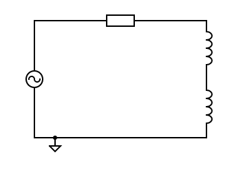
Figure 2: Electric circuit with voltage source, resistor and two inductors.

1.a. This is modeled with a component-wise approach using ModelingToolkitStandardLibrary. The resulting model has 28 equations and 29 variables.

using ModelingToolkit, JuliaSimControl, OrdinaryDiffEq
using ModelingToolkitStandardLibrary.Electrical
using ModelingToolkitStandardLibrary.Blocks
using Plots

@parameters t

# Defining the parameters:
R = 4.0
L = 6.0
V = 12.0

# Defining the components and connections:
@named R1 = Resistor(; R = R)
@named L1 = Inductor(; L = 0.5*L)
@named L2 = Inductor(; L = 0.5*L )
@named voltage = Voltage()
@named input = RealInput()
@named output = RealOutput()
@named ground = Ground()
rl_source_eqns = [
        Symbolics.connect(input, voltage.V)
        Symbolics.connect(voltage.p, R1.p)
        Symbolics.connect(R1.n, L1.p)
        Symbolics.connect(L1.n, L2.p)
        Symbolics.connect(L2.n, voltage.n)
        Symbolics.connect(ground.g, voltage.n)
        output.u ~ L2.i
        ]

# Defining the DAE system
@named circuit_dae = ODESystem(rl_source_eqns, t, systems=[R1, L1, L2, voltage, input, output, ground])

\[ \begin{equation} \left[ \begin{array}{c} output_{+}u\left( t \right) = L2_{+}i\left( t \right) \\ \mathrm{connect}\left( input, voltage_{+}V \right) \\ \mathrm{connect}\left( voltage_{+}p, R1_{+}p \right) \\ \mathrm{connect}\left( R1_{+}n, L1_{+}p \right) \\ \mathrm{connect}\left( L1_{+}n, L2_{+}p \right) \\ \mathrm{connect}\left( L2_{+}n, voltage_{+}n \right) \\ \mathrm{connect}\left( ground_{+}g, voltage_{+}n \right) \\ R1_{+}v\left( t \right) = R1_{+}p_{+}v\left( t \right) - R1_{+}n_{+}v\left( t \right) \\ 0 = R1_{+}n_{+}i\left( t \right) + R1_{+}p_{+}i\left( t \right) \\ R1_{+}i\left( t \right) = R1_{+}p_{+}i\left( t \right) \\ R1_{+}v\left( t \right) = R1_{+}R R1_{+}i\left( t \right) \\ L1_{+}v\left( t \right) = L1_{+}p_{+}v\left( t \right) - L1_{+}n_{+}v\left( t \right) \\ 0 = L1_{+}p_{+}i\left( t \right) + L1_{+}n_{+}i\left( t \right) \\ L1_{+}i\left( t \right) = L1_{+}p_{+}i\left( t \right) \\ \frac{\mathrm{d} L1_{+}i\left( t \right)}{\mathrm{d}t} = \frac{L1_{+}v\left( t \right)}{L1_{+}L} \\ L2_{+}v\left( t \right) = L2_{+}p_{+}v\left( t \right) - L2_{+}n_{+}v\left( t \right) \\ 0 = L2_{+}n_{+}i\left( t \right) + L2_{+}p_{+}i\left( t \right) \\ L2_{+}i\left( t \right) = L2_{+}p_{+}i\left( t \right) \\ \frac{\mathrm{d} L2_{+}i\left( t \right)}{\mathrm{d}t} = \frac{L2_{+}v\left( t \right)}{L2_{+}L} \\ voltage_{+}v\left( t \right) = voltage_{+}p_{+}v\left( t \right) - voltage_{+}n_{+}v\left( t \right) \\ 0 = voltage_{+}p_{+}i\left( t \right) + voltage_{+}n_{+}i\left( t \right) \\ voltage_{+}i\left( t \right) = voltage_{+}p_{+}i\left( t \right) \\ voltage_{+}v\left( t \right) = voltage_{+}V_{+}u\left( t \right) \\ ground_{+}g_{+}v\left( t \right) = 0 \\ \end{array} \right] \end{equation} \]

1.b. Optionally, the user may simplify the system. The voltage is set as a control input in the inputs array:

inputs = [input.u]
outputs = []
sys, diff_idxs, alge_idxs, input_idxs = ModelingToolkit.io_preprocessing(circuit_dae, inputs, outputs)
sys

\[ \begin{align} \frac{\mathrm{d} L2_{+}i\left( t \right)}{\mathrm{d}t} =& L1_{+}iˍt\left( t \right) \\ 0 =& R1_{+}v\left( t \right) + L2_{+}v\left( t \right) - voltage_{+}V_{+}u\left( t \right) + L1_{+}v\left( t \right) \end{align} \]

After simplification, the system becomes a DAE with 1 algebraic equation, 1 ordinary differential equation, 2 states and 1 control input.

1.c. After simplification, one may simulate the DAE using a suitable algorithm such as Rodas4().

tspan = (0.0, 10.0)
x0 = Dict(
    L1.p.i => 0.0,
    L2.v => 0.0,
)
u0 = Dict(
    input.u => 12.0
)
prob = ODEProblem(sys, x0, tspan, u0, jac = true)
sol = solve(prob, Rodas4())
plot(sol, idxs = [L1.i, L2.v])

1. To determine the trim point, here we set a desired current in the circuit, and call the trim function:

desired_states = Dict(L1.i => 9.0)
sol, trim_states = trim(circuit_dae; inputs, outputs, desired_states)
trim_states[L1.i]

8.999999988737004

Index

• JuliaSimControl.trim

trim(sys::AbstractSystem;
    inputs = [], outputs = [], params = Dict(),
    desired_states = Dict(), hard_eq_cons = Equation[], soft_eq_cons = Equation[], hard_ineq_cons = Inequality[], soft_ineq_cons = Inequality[], 
    penalty_multipliers = Dict(:desired_states => 1.0, :trim_cons => 1.0, :sys_eqns => 10.0), dualize = false,
    solver = IPNewton(), verbose = false, simplify = false, kwargs...)