Robust control

Robust control refers to a set of design and analysis methods that attempt to guarantee stability and performance of a closed-loop control system in the presence of uncertainties, such as plant model mismatch and unknown disturbances.

JuliaSimControl provides a wide set of tools to facilitate robust-control workflows:

Robust control

Analysis

Structured singular value and diskmargin

Examples

Synthesis

Examples

Robust MPC

See examples

Uncertainty modeling

Uncertainty modeling is a key step in robust-control workflows. RobustAndOptimalControl.jl provides a set of tools to facilitate modeling both parametric and unstructured uncertainty for linear systems.

Examples

Uncertainty modeling for nonlinear systems

When working with nonlinear models, defined in ModelingToolkit or as a differential equation, we have the following options for uncertainty modeling:

Parametric uncertainty

The simplest method is to model uncertainty in one or several parameters (including initial conditions) and perform Monte-Carlo simulations to propagate the uncertainty to the output quantity of interest. Below is an example where a mass-spring-damper is modeled with an uncertain spring stiffness using MonteCarloMeasurements.jl.

using ModelingToolkit, MonteCarloMeasurements, Plots, OrdinaryDiffEq
T = typeof(1 ± 1)
@parameters t k::T d
@variables x(t)::T v(t)::T
D = Differential(t)
eqs = [D(x) ~ v, D(v) ~ -k*x - d*v - 9.82]
@named sys = ODESystem(eqs, t)
prob = ODEProblem(complete(sys), [x => 0.0 ± 0.1, v => 0.0, k => 10 ± 1, d => 1], (0.0, 10.0))
sol = solve(prob, Tsit5())
plot(sol, ri=false, N=1000) # ribbon = false and plot 1000 sample trajectories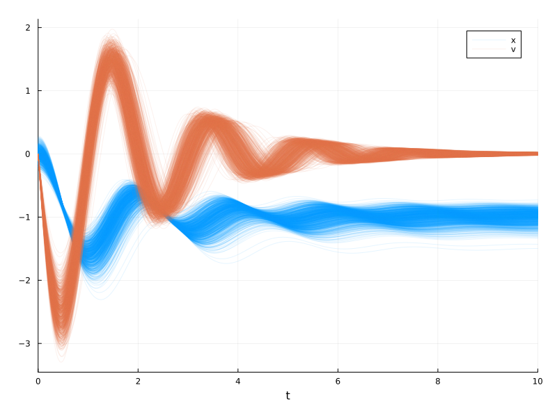

In this example, we provided the initial condition x => 0.0 ± 0.1 and the spring stiffness k => 10 ± 1. The μ ± σ operator is defined by MonteCarloMeasurements.jl and defaults to creating 2000 samples from a normal distribution. However, we are no limited to normal distributions, and can use any other distribution or manually selected samples.

Interval and set propagation methods

Unstructured uncertainty

For linear systems, we have powerful tools for the modeling and analysis of systems with unstructured uncertainty, such as neglected or missing dynamics. When dealing with nonlinear systems, we can approach the problem in a similar way, either by linearizing the system and making use of the linear tools, or by attempting to translate the problem into a problem of parametric uncertainty. To linearize a nonlinear system, see Linear analysis, during the rest of this section, we will focus on the parametric uncertainty approach.

A common model for lumped uncertainty from linear robust control is multiplicative uncertainty (relative uncertainty). We can view such an uncertainty model in a block diagram

                  ┌────┐   
                ┌►│ WΔ ├┐  
                │ └────┘│  
  ┌───┐   ┌───┐ │       ▼  
┌►│ C ├──►│ P ├─┴───────+─►y
│ └───┘   └───┘         │  
│                       │  
└───────────────────────┘

here, $\Delta : ||\Delta|| < 1$ is a norm-bounded uncertain element, $W$ is a known dynamic scaling, and $P$ and $C$ represent the plant and controller, respectively. The scaling system $W$ is chosen such to be large when the relative uncertainty is large, typically in a frequency-dependent manner. For example, if we trust the model for low frequencies but are uncertain about the high frequencies, we can choose $W$ to be a linear system that looks something like this

using JuliaSimControl, Plots
W = makeweight(0.1, 1, 0.9)
bodeplot(W, plotphase=false, title="Scaling of uncertainty, \$W(s)\$")

this indicates that we have a 10% uncertainty in the low frequencies, and a 90% uncertainty for high frequencies. All we know about the uncertain element $\Delta$ is that it has a norm bounded by 1. To be able to simulate in the presence of this uncertain element, we can draw several samples of $\Delta$ and simulate with all of them. Continuing the mass-spring-damper example from above, we consider $y = x(1+WΔ)$ to be the uncertain output.

using ControlSystemsMTK
T = typeof(-1..1)
@parameters Δ::T=(-1..1) # The uncertain element is between -1 and 1
@variables y(t)

@named Wsys = ODESystem(W)

connections = [
    Wsys.input.u ~ sys.x
    y ~ sys.x + Wsys.output.u*Δ
]

@named uncertain_sys = ODESystem(connections, t, systems=[sys, Wsys])
initial_condition = [sys.x => zero(T), sys.v => 0.0, sys.k => T(10), sys.d => 1]
prob = ODEProblem(structural_simplify(uncertain_sys, split=false), initial_condition, (0.0, 10.0))
sol = solve(prob, Tsit5())
plot(sol, ri=false, N=500, idxs=[sys.x, sys.v, y], layout=2, sp=[1 2 1], l=[3 3 1]) # ribbon = false and plot 500 sample trajectories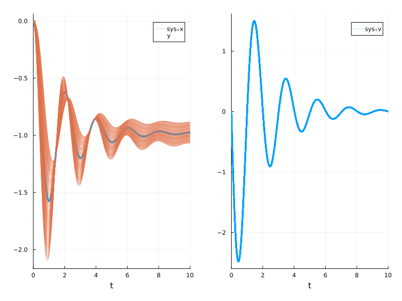

This time, we had no uncertainty in the spring coefficient, instead we had a large uncertainty when the system was operating in the high-frequency region. We see this in the figure above, the uncertainty is large during the transient, but significantly smaller after having reached steady-state.

This method of translating the problem of modeling unstructured uncertainty into parametric uncertainty is very general, and can easily be adapted to, e.g., situations in which dynamics is either present or not by letting $\Delta \in \{0, 1\}$ instead of $\Delta \in [-1, 1]$.