Control design for a quadruple-tank system with JuliaSim Control
In this example, we will implement several different controllers of increasing complexity for a nonlinear MIMO process, starting with a PID controller and culminating with a nonlinear MPC controller with state and input constraints.
This example has an associated video where we provide additional context and insights:
The process we will consider is a quadruple tank, where two upper tanks feed into two lower tanks, depicted in the schematics below. The quad-tank process is a well-studied example in many multivariable control courses, this particular instance of the process is borrowed from the Lund University introductory course on automatic control.
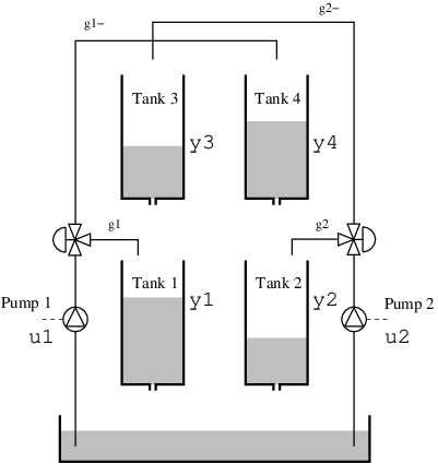
The process has a cross coupling between the tanks, governed by a parameters $\gamma_i$: The flows from the pumps are divided according to the two parameters $γ_1 , γ_2 ∈ [0, 1]$. The flow to tank 1 is $γ_1 k_1u_1$ and the flow to tank 4 is $(1 - γ_1 )k_1u_1$. Tanks 2 and 3 behave symmetrically.
The dynamics are given by
\[\begin{aligned} \dot{h}_1 &= \dfrac{-a_1}{A_1} \sqrt{2g h_1} + \dfrac{a_3}{A_1} \sqrt{2g h_3} + \dfrac{γ_1 k_1}{A_1} u_1 \\ \dot{h}_2 &= \dfrac{-a_2}{A_2} \sqrt{2g h_2} + \dfrac{a_4}{A_2} \sqrt{2g h_4} + \dfrac{γ_2 k_2}{A_2} u_2 \\ \dot{h}_3 &= \dfrac{-a_3}{A_3} \sqrt{2g h_3} + \dfrac{(1-γ_2) k_2}{A_3} u_2 \\ \dot{h}_4 &= \dfrac{-a_4}{A_4} \sqrt{2g h_4} + \dfrac{(1-γ_1) k_1}{A_4} u_1 \end{aligned}\]
where $h_i$ are the tank levels and $a_i, A_i$ are the cross-sectional areas of outlets and tanks respectively. For this system, if $0 \leq \gamma_1 + \gamma_2 < 1$ the system is non-minimum phase, i.e., it has a zero in the right half plane.
In the examples below, we assume that we can only measure the levels of the two lower tanks, and need to use a state observer to estimate the levels of the upper tanks.
The interested reader can find more details on the quadruple-tank process from the manual provided here (see "lab 2"), from where the example is taken.
We will consider several variants of the MPC controller:
- Linear control using a PID controller.
- Linear MPC with a linear observer and prediction model.
- MPC with a linear prediction model but a nonlinear observer.
- Linear MPC with integral action and output references.
- Nonlinear MPC using a nonlinear observer and prediction model.
In all cases we will consider constraints on the control authority of the pumps as well as the levels of the tanks.
We start by defining the dynamics:
using DyadControlSystems
using DyadControlSystems.MPC
using StaticArrays
using Plots, Plots.Measures, LinearAlgebra
using Test

## Nonlinear quadtank
const kc = 0.5
function quadtank(h, u, p = nothing, t = nothing)
    k1, k2, g = 1.6, 1.6, 9.81
    A1 = A3 = A2 = A4 = 4.9
    a1, a3, a2, a4 = 0.03, 0.03, 0.03, 0.03
    γ1, γ2 = 0.2, 0.2

    ssqrt(x) = √(max(x, zero(x)) + 1e-3) # For numerical robustness at x = 0

    xd = SA[
        -a1 / A1 * ssqrt(2g * h[1]) + a3 / A1 * ssqrt(2g * h[3]) + γ1 * k1 / A1 * u[1]
        -a2 / A2 * ssqrt(2g * h[2]) + a4 / A2 * ssqrt(2g * h[4]) + γ2 * k2 / A2 * u[2]
        -a3 / A3 * ssqrt(2g * h[3]) + (1 - γ2) * k2 / A3 * u[2]
        -a4 / A4 * ssqrt(2g * h[4]) + (1 - γ1) * k1 / A4 * u[1]
    ]
end

nu = 2 # number of control inputs
nx = 4 # number of states
ny = 2 # number of measured outputs
Ts = 2 # sample time
w = exp10.(-3:0.1:log10(pi / Ts)) # A frequency-vector for plotting

discrete_dynamics0 = rk4(quadtank, Ts, supersample = 2) # Discretize the nonlinear continuous-time dynamics
state_names = :h^4
measurement = (x, u, p, t) -> kc * x[1:2]
discrete_dynamics =
    FunctionSystem(discrete_dynamics0, measurement, Ts, x = state_names, u = :u^2, y = :h^2)
FunctionSystem{Discrete{Int64}, SeeToDee.Rk4{typeof(Main.quadtank), Float64}, Main.var"#2#3", Vector{Symbol}, Vector{Symbol}, Vector{Symbol}, Nothing, UnitRange{Int64}, SciMLBase.NullParameters, UnitRange{Int64}, Nothing}(SeeToDee.Rk4{typeof(Main.quadtank), Float64}(Main.quadtank, 2.0, 2), Main.var"#2#3"(), Discrete{Int64}(2), [:h1, :h2, :h3, :h4], [:u1, :u2], [:h1, :h2], nothing, 1:4, SciMLBase.NullParameters(), 0:-1, nothing)Next, we define the constraints and an operating point. The maximum allowed control signal will be determied by an interactive slider that is placed further down in the notebook. We start by defining a desired state at the operating point, xr0
xr0 = [10, 10, 6, 6]; # desired reference stateWe then solve for the state and control input that is close to the desired state and yields a stationary condition (zero derivative
xr, ur = begin # control input at the operating point
    using Optim
    optres = @views Optim.optimize(
        xu ->
            sum(abs, quadtank(xu[1:4], xu[5:6], 0, 0)) + 0.0001sum(abs2, xu[1:4] - xr0),
        [xr0; 0.25; 0.25],
        BFGS(),
        Optim.Options(iterations = 100, x_tol = 1e-7),
    )
    @info optres
    optres.minimizer[1:4], optres.minimizer[5:6]
end
([9.821807570823184, 9.821748135033353, 6.2859416106655885, 6.285891656375277], [0.26028358713924393, 0.2602828992285937])# Control limits
umin = fill(0.0, nu)
umax = fill(0.6, nu)
# State limits
xmin = zeros(nx)
xmax = Float64[12, 12, 8, 8]
constraints_pid = MPCConstraints(; umin, umax, xmin, xmax)
x0 = [2, 1, 8, 3] # Initial tank levels
Cc, Dc = DyadControlSystems.linearize(measurement, xr, ur, 0, 0)
op = OperatingPoint(xr, ur, Cc * xr)OperatingPoint{Vector{Float64}, Vector{Float64}, Vector{Float64}}([9.821807570823184, 9.821748135033353, 6.2859416106655885, 6.285891656375277], [0.26028358713924393, 0.2602828992285937], [4.910903785411592, 4.910874067516676])PID control
Our first attempt at controlling the level in the quad-tank system is going use a PID controller. We will tune the controller using the automatic tuning capabilities of DyadControlSystems. To make use of the autotuner, we need a linearized model of the plant, for which we make use of the function linearize.
disc(x) = c2d(ss(x), Ts) # Discretize the linear model using zero-order-hold

Ac, Bc = DyadControlSystems.linearize(quadtank, xr, ur, 0, 0)
Cc, Dc = DyadControlSystems.linearize(measurement, xr, ur, 0, 0)
Gc = ss(Ac, Bc, Cc, Dc)

G = disc(Gc)
Since this is a MIMO system and PID controllers are typically SISO, we look for an input-output pairing that is approximately decoupled. To this end, we investigate the relative-gain array (RGA). If we aim for a crossover bandwidth of around 0.01rad/s, we find the optimal input-output pairings for decoupled PID control using the relative gain array:
relative_gain_array(Gc, 0.01) .|> abs2×2 Matrix{Float64}:
0.235216 0.851678
0.851678 0.235216Unfortunately, this matrix is rather far from diagonalizable using permutations, indicating that there is a somewhat strong cross-coupling in the system and standard PID control is likely to be difficult (the parameter $\gamma$ directly influeces the cross-coupling). Investigating the RGA as a function of frequency, we further notice that for high frequencies, the conclusion about the input-output pairing changes!
rgaplot(
    Gc,
    w,
    legend = false,
    layout = 4,
    plot_title = "RGA plot",
    title = "",
    ylabel = "",
    grid = false,
    link = :both,
)
In our case, we will stick with the pairing we decided upon for low frequencies, since the input and state constraints will limit how fast we can control the system. We proceed to tune a controller for the $u_1 \rightarrow y_2$ mapping and do this by defining an AutoTuningProblem. This approach lets us put constraints on the largest magnitude of the closed-loop sensitivity functions, $M_S, M_T, M_{KS}$.
tuningprob = AutoTuningProblem(;
    P = Gc[2, 1],
    Ts,
    w = exp10.(LinRange(-4, -1, 100)),
    Ms = 1.1,
    Mt = 1.05,
    Mks = 20,
    Tf = 1200,
    metric = :IAE,
)
We solve the problem by calling solve
tuningresult = solve(tuningprob, xtol_rel = 1e-4)┌ Warning: Unable to balance state-space, returning original system
└ @ ControlSystemsBase ~/.julia/packages/ControlSystemsBase/F0bxl/src/types/conversion.jl:166
┌ Warning: Unable to balance state-space, returning original system
└ @ ControlSystemsBase ~/.julia/packages/ControlSystemsBase/F0bxl/src/types/conversion.jl:166
┌ Warning: Unable to balance state-space, returning original system
└ @ ControlSystemsBase ~/.julia/packages/ControlSystemsBase/F0bxl/src/types/conversion.jl:166
┌ Warning: Unable to balance state-space, returning original system
└ @ ControlSystemsBase ~/.julia/packages/ControlSystemsBase/F0bxl/src/types/conversion.jl:166
┌ Warning: Unable to balance state-space, returning original system
└ @ ControlSystemsBase ~/.julia/packages/ControlSystemsBase/F0bxl/src/types/conversion.jl:166
┌ Warning: Unable to balance state-space, returning original system
└ @ ControlSystemsBase ~/.julia/packages/ControlSystemsBase/F0bxl/src/types/conversion.jl:166The autotuning returns a result structure, the PID+filter parameters are available as tuningresult.p while a controller object is available as tuningresult.K. One can further call OptimizedPID(tuningresult) to obtain a ModelingToolkit system that represents the tuned controller including anti-windup etc.
tuningresult.p4-element Vector{Float64}:
0.1154040387893927
0.0003779077091614526
9.281798110751033
10.000000775540606plot(tuningresult, titlefont = 9)
xlims!((-5, 1), ylims = (-5, 0.5), sp = 4, legend = :bottomleft);
The resulting controller respects the sensitivity constraints, visualized in both Bode plots and the Nyquist plot as dashed lines.
We also construct a static precompensator iG0 = $G(0)^{-1}$ that decouples the system at DC. This strategy can sometimes mitigate the problem with cross-coupling between the channels, but may be treacherous if the relative-gain array contains large entries (which is fortunately not the case in our problem).
iG0 = [0 1; 1 0] # No decouplingWe form the final controller by applying the static precompensator $G_0^{-1}$ to the optimized PID controller
Cpid = (tuningresult.K * I(2)) * iG0;To increase the realism in the simulation of the final system, we add the saturation nonlinearity that corresponds to actuator limitations, as well as the offsets implied by the linearization point to get the correct units on the signals:
using ControlSystemsBase: offset, saturation
Gcop = offset(op.y) * Gc * offset(-op.u)
Cpid_sat = saturation(constraints_pid.umin, constraints_pid.umax) * Cpid
The simulation of the closed-loop system controlled by the PID controller is shown belo
fig1 = plot(
    lsim(feedback(Gcop * Cpid_sat), Gc.C * xr, 0:Ts:1500, x0 = [x0 - op.x; zeros(Cpid.nx)]),
    layout = 1,
    sp = 1,
    title = "Outputs",
    ylabel = "",
)
hline!(Gc.C * xr, l = :dash, c = 1, legend = false)
plot(
    fig1,
    plot(
        lsim(
            feedback(Cpid_sat, Gcop),
            Gc.C * xr,
            0:Ts:1500,
            x0 = [zeros(Cpid.nx); x0 - op.x],
        ),
        layout = 1,
        sp = 1,
        title = "Control signals",
        ylabel = "",
    ),
    size = (1000, 300),
    margin = 4mm,
)
The result looks alight, but the problems are multiple:
- The input saturation causes the control signal to frequently hit the control limits and we thus effectively loose feedback during large transients.
- The rather large cross-coupling between the channels is mostly ignored by the PID controller.
- The non-measured states that were not allowed to go above certain levels overshot this constraint, shown below.
res_pid =
    lsim(feedback(Gcop * Cpid_sat), Gc.C * xr, 0:Ts:1000, x0 = [x0 - op.x; zeros(Cpid.nx)])
sfig = plot(
    res_pid.t,
    res_pid.x[1:4, :]' .+ op.x',
    label = string.(permutedims(:x^4)),
    title = "States and constraints",
    layout = 4,
)
plot!(OvershootObjective.(constraints_pid.xmax), sp = (1:4)')
sfig
This demonstrates that it can be treacherous to rely on optimization without taking all aspects of the problem into account. Furthermore, In order to successfully control the tank system and respect input and state constraints using a PID controller, we would have to accept a lower performance, e.g., by lowering the constraint $M_{KS}$ in the autotuning problem.
Fortunately, the MPC framework is very capable of taking input and state consstraints into account, something we will explore soon.
Robustness analysis
The quadtank being a MIMO system means that the classical gain and phase margins are somewhat hard to apply. A robustness measure that is more suitable to the MIMO setting that also tells you something about simultaneous perturbations to both gain and phase at the plant input is the diskmargin and disk-based gain and phase margins, which we may plot as a function of frequency:
plot(diskmargin(Gc, Cpid, 0, w).simultaneous_input);
ylims!((1, 8), sp = 1, yscale = :identity, legend = false);
dm_pid = diskmargin(Cpid * Gc)Disk margin with:
Margin: 0.8038277922776178
Frequency: 0.009417766006869529 rad/s, 0.0014988840128761062 Hz
Gain margins: [0.4266211395068248, 2.3440001148466356]
Phase margin: 43.79175991949295
Delay margin: 81.15623124215804 s
Skew: 0
Worst-case perturbation: missing
We see that we have modest gain and phase margins, certainly not too impressive. Keep in mind, that these margins assumes a linear system without, e.g., the input saturation.
We may also visualize the stable region in the plane of simultaneous gain and phase variations:
plot(dm_pid)
Linear MPC
With a MPC controller, we can take the constraints into account explicitly in the optimization problem solved at each sample time.
In some situations, we may want to resort to a linear MPC controller. A linear controller is often sufficient when the task is regulation, i.e., keeping a controlled variable at a fixed set point.
We proceed in a similar fashion to above, making use of the model linearized around the specified operating point $(x_r,u_r,y_r)$. We also construct a Kalman filter for state estimation.
For a linear MPC controller to work well, we must provide the operating point around which we have linearized. We also construct a LinearMPCModel that keeps track of the model and it's operating point
constraints_lmpc = MPCConstraints(; umin, umax, xmin, xmax)

R1 = 1e-5 * I(nx) # Dynamics covariance
R2 = I(ny)      # Measurement covariance

kf_lmpc = let (A, B, C, D) = ssdata(G)
    KalmanFilter(A, B, C, D, R1, R2)
end
pm = LinearMPCModel(
    G,
    kf_lmpc;
    constraints = constraints_lmpc,
    op,
    x0,
    strictly_proper = false,
)
We also specify some cost matrices for the MPC problem and the prediction horizon $N$. We will later see how to choose these matrices in more principled ways
N = 10 # Prediction horizon
Q1 = 1.0 * I(nx)
Q2 = 1.0 * I(nu)
qs = 100
qs2 = 100000
Let's simulate the linear MPC:
solver = OSQPSolver(
    eps_rel = 1e-5,
    eps_abs = 1e-4,
    max_iter = 5000,
    check_termination = 5,
    verbose = false,
    sqp_iters = 1,
    polish = true, # to get high accuracy
)

prob_lin = LQMPCProblem(
    pm;
    Q1,
    Q2 = 0Q2,
    Q3 = Q2,
    qs,
    qs2,
    N,
    r = xr,
    solver,
)

@time hist_lin = MPC.solve(
    prob_lin;
    x0,
    T = 1000 ÷ Ts,
    verbose = false,
    noise = 0,
    dyn_actual = discrete_dynamics,
)
plot(hist_lin, plot_title = "Linear MPC", legend = :bottomright)
The controller performs reasonably well and respects the input constraints. We notice that the control-signal trajectory looks qualitatively different now compared to when the PID controller was used, in particular during the time when the state constraints are active for the upper tanks.
With a linear observer, we notice a slight violation of the state constraints for states $h_3, h_4$, remember, we do not measure these states directly, rather we rely on the observer to estimate them. Due to the square root in the dynamics that govern the outflow of liquid from the tanks, the observer thinks that the outflow is greater than it actually is at levels well above the linearization point.
In practice, it's unrealistic to assume that we know the static gain of the system perfectly, in fact, the static gain for this system probably varies with the temperature of the equipment, the tank contents and during the lifetime of the tanks and pumps. We would thus likely end up with a stationary error using the controller above. This highlights a problem with naive MPC control (and similarly for standard LQG control), we do not have any integral action in the controller! We will soon see how we can add integral action, but first we explore how we can make use of a nonlinear observer (EKF) together with a linear prediction model in order to improve the constraint satisfaction.
Linear MPC with nonlinear observer
The nonlinear observer will make use of an extended Kalman filter (EKF). When we use a nonlinear observer together with a linear prediction model, we must adjust the inputs and outputs of the observer to account for the fact that the prediction model operates in $\Delta$-coordinates. We do this using an OperatingPointWrapper.
kf_ekf = let
    A, B, C, D = ssdata(G)
    KalmanFilter(A, B, C, D, R1, R2)
end
ekf =
    ExtendedKalmanFilter(kf_ekf, discrete_dynamics.dynamics, discrete_dynamics.measurement)
To highlight the problem of lacking integral action, we throw an input disturbance into the mix. The disturbance simulates a leakage in the pump after 500s.
function disturbance(u, t)
    t > 500 / Ts ? [-0.02, 0] : [0.0, 0]
end
pm_ekf = LinearMPCModel(
    G,
    DyadControlSystems.OperatingPointWrapper(ekf, op);
    constraints = constraints_lmpc,
    op,
    x0,
    strictly_proper = false,
)
prob_ekf = LQMPCProblem(
    pm_ekf;
    Q1,
    Q2 = 0Q2,
    Q3 = Q2,
    qs,
    qs2,
    N,
    r = xr,
    solver,
)
@time hist_ekf =
    MPC.solve(prob_ekf; x0, T = 1000 ÷ Ts, dyn_actual = discrete_dynamics, disturbance)
plot(hist_ekf, plot_title = "Linear MPC with nonlinear observer", legend = :bottomright)
vline!([500], lab="Disturbance start", l=(:red, :dash))
With the nonlinear observer, we notice that the violation of the soft state constraints is eliminated. This is an indication that the estimation of the states is more accurate compared to when we used a standard Kalman filter. We do, however, fail to reject the constant disturbance due the the lack of integral action in the controller.
Integral action and robust tuning
Finally, we explore how to add integral action to the controller. We will make use of a loop-shaping strategy, where we "shape" the linearized plant $G$ with a PI controller at the inputs.
W1 = tf(0.001 * [100, 1], [1, 1e-6]) |> disc # "Shape" the plant with a PI-controller (the 1e-6 is for numerical robustness)
W1 = (W1 * I(2)) * iG0 # Make the PI-controller 2×2 since we have 2 inputs
When performing loop shaping, it's helpful to inspect the singular value plot of the loop-transfer function. Below, we show the singular values for the open-loop plant, the shaped plant and the resulting robustified plant.
sigmaplot(
    [G, G * W1],
    w,
    lab = ["Plant" "Loop-shaped plant"],
)
The parameters of $W_1$ were chosen so as to get a reasonable loop shape. The construction of the RobustMPCModel will give a warning if the resulting controller has poor robustness in the sense of the normalized co-prime margin (see ncfmargin and glover_mcfarlane for more details, the $\gamma$ value is available as model.gmf[2]).
Since this is a linear controller with a linear observer, we once again adjust the constraints to the operating point. We now create a RobustMPCModel where we provide the loop-shaping controller $W_1$. Internally, this makes use of the Glover-McFarlane method to find a robust controller and inverse optimal control to find the optimal cost matrices $Q_1, Q_2$.
This example also makes use of output references rather than the earlier state references. We thus say state_reference = false when we create the model, and provide op.y as reference to the problem constructor.
model = RobustMPCModel(
    G;
    W1,
    constraints = constraints_lmpc,
    x0,
    op,
    K = kf_lmpc,
)

prob_roby =
    LQMPCProblem(model; qs, qs2, N, r = op.y, solver)

@time hist_roby = MPC.solve(
    prob_roby;
    x0,
    T = 1500 ÷ Ts,
    verbose = false,
    noise = 0,
    dyn_actual = discrete_dynamics,
    Cz_actual = G.C, # Indicate the outputs of the actual dynamics used to measure performance
    disturbance,
)

plot(hist_roby, plot_title = "Robust LMPC with output reference", legend = :bottomright)
vline!([500], lab="Disturbance start", l=(:red, :dash))
The soft state-constraints are not fully respected; since the observer uses a linearized model, it fails to estimate the true value of the state and the actual value might thus be violating the constraints slightly. The figure above shows state trajectories, we may plot also the output trajectories to verify that the output reference was met without steady-state tracking error:
plot(
    hist_roby,
    ploty = true,
    plot_title = "Robust LMPC with output reference",
    legend = :bottomright,
)
vline!([500], lab="Disturbance start", l=(:red, :dash))
thanks to the integrator in the controller, we now manage to reach the reference without steady-state error!
We can look at the loop shape for the robustified controller as well
sigmaplot(
    [G, G * W1, G * model.gmf[1]],
    w,
    lab = ["Plant" "Loop-shaped plant" "Robust loop gain"],
)
the change is non-trivial and likely nothing that would have been feasible reasching by manual loop shaping!
Robustness analysis
Also for the linear MPC regulator can we analyze robustness properties (assuming no constraints are active). We plot the multivariable diskmargins like we did for the PID controller above. The linear controller that is equivalent to the MPC controller, abscent constraints, is available in the model object
equivalent_controller = model.gmf[1]
f1 = plot(
    diskmargin(G, equivalent_controller, 0, w).simultaneous_input,
    lower = false,
    label = "Simultaneous perturbations",
)
plot!(
    diskmargin(G, equivalent_controller, 0, w).input[1],
    lower = false,
    label = "Single channel perturbation",
    legend = false,
)
ylims!((1, 12), sp = 1, yscale = :identity)
ylims!((-Inf, 100), sp = 2, yscale = :identity)
plot!(legend = :right, sp = 1)
plot(
    f1,
    plot(diskmargin(equivalent_controller * G, 0), titlefont = 10),
    size = (900, 400),
    margin = 5mm,
)
diskmargin(equivalent_controller * G)Disk margin with:
Margin: 0.6343119070309075
Frequency: 0.009682153059967075 rad/s, 0.0015409625192660803 Hz
Gain margins: [0.5184230801690975, 1.9289264661477326]
Phase margin: 35.19346854907748
Delay margin: 63.44063118751836 s, 31 samples
Skew: 0
Worst-case perturbation: missing
The margins obtained above depend somewhat on the decoupler $G(0)^{-1}$ that we chose, but are better than for the PID controller, even though the PID controller was optimized for robustness. We should keep in mind that the margins we consider here pertaines to simultaneous perturbations at both input channels, and we have thus in essence added twice the perturbation compared to what we would have done in a SISO setting. We may also ask the robust MPC model for its normalized-coprime-factor (NCF) margin:
model.info.margin0.3056115549407793An NCF margin larger than about 0.25-0.3 indicates a successful and robust design.
Nonlinear MPC
The last controller we'll consider is a nonlinear MPC controller that uses the nonlinear model of the plant for prediction, paired with a nonlinear observer. We will make use of the extended Kalman filter we defined above.
solver_nl = OSQPSolver(
    eps_rel = 1e-6,
    eps_abs = 1e-5,
    max_iter = 50000,
    check_termination = 5,
    sqp_iters = 3,
    dynamics_interval = 1,
    verbose = false,
    polish = true,
)
constraints = NonlinearMPCConstraints(; xmin, xmax, umin, umax)
prob_nl = QMPCProblem(
    discrete_dynamics;
    observer = ekf,
    Q1,
    Q2,
    qs = 0,
    qs2 = 0,
    constraints = constraints,
    N,
    xr,
    ur,
    solver = solver_nl,
)

@time hist_nl = MPC.solve(prob_nl; x0, T = 1000 ÷ Ts, verbose = false, noise = 0)
plot(hist_nl, plot_title = "Nonlinear MPC")
Let's test that the state converged to our reference and that the constraints were met.
@test hist_nl.X[end] ≈ xr atol = 0.1

U = reduce(hcat, hist_nl.U)
@test all(maximum(U, dims = 2) .< umax .+ 1e-2)
@test all(minimum(U, dims = 2) .> umin .- 1e-2)
Test PassedAs we can see, the nonlinear MPC controller performs quite well and respects the state constraints.
Summary
We have seen how to
- tune PID controllers automatically
- define and simulate MPC controllers
- analyze robustness of feedback systems