Getting started with linear control

This page will guide the user through how build and manipulate linear models, and to perform linear control design for a simple system in multiple different ways.

Getting started with linear control

More detailed tutorials on each topic are available in the tutorials section.

Linear models

Linear models are built and manipulated using the tools from ControlSystems.jl and RobustAndOptimalControl.jl. See the documentation on creating and manipulating systems to get started.

Time and frequency domain analysis of linear systems

See Time and frequency response analysis to get started.

Analysis of linear systems

To get started with classical robustness analysis of linear systems, see Analysis of linear control systems as well as the video below.

Design examples: The system model

The following sections include introductory examples to get you started with linear control design. Throughout, we will consider a simple model of two masses connected by a spring and a viscous damper, depicted below. 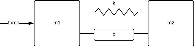Double-mass model

This model is predefined in the module DemoSystems:

using JuliaSimControl, Plots
P = DemoSystems.double_mass_model() # The function `double_mass_model` returns a `StateSpace` object

StateSpace{Continuous, Float64}
A = 
    0.0   1.0     0.0   0.0
 -100.0  -2.0   100.0   1.0
    0.0   0.0     0.0   1.0
  100.0   1.0  -100.0  -2.0
B = 
 0.0
 1.0
 0.0
 0.0
C = 
 1.0  0.0  0.0  0.0
D = 
 0.0

Continuous-time state-space model

We can plot its Bode plot using bodeplot

bodeplot(P) # See https://juliaplots.org/ for more information on plotting

PID control

PID: Manual tuning

A PID controller can be created using the function pid

using JuliaSimControl, Plots
P = DemoSystems.double_mass_model()

C = pid(5, 1, 1, Tf=0.01)         # The keyword argument `Tf` specifies the time constant for a lowpass filter.
Gcl = feedback(P*C)               # We can form the closed-loop system from reference to output using [`feedback`](@ref)
f1 = bodeplot([P*C, Gcl], lab=["PC" "" "PC/(1+PC)" ""]) # We plot the Bode curve of the loop-transfer function and the closed-loop transfer function
f2 = plot(step(Gcl, 0:0.01:10))   # And plot a step response
plot(f1,f2)                       # Combine to plots in a single figure

Functions used:

See also the video below, where a simple PID controller is designed for the double-mass model, and the robustness properties of the closed-loop system are analyzed.

PID: Automatic tuning

PID controllers can be tuned automatically by specifying and solving an AutoTuningProblem. See PID Autotuning for more details.

using JuliaSimControl, Plots
P = DemoSystems.double_mass_model()

# Robustness constraints
Ms = 1.3     # Maximum allowed sensitivity function magnitude
Mt = Ms      # Maximum allowed complementary sensitivity function magnitude
Mks = 1000.0 # Maximum allowed magnitude of transfer function from process output to control signal, sometimes referred to as noise sensitivity.
w = 2π .* exp10.(LinRange(-2, 2, 200)) # Frequency grid
Ts = 0.005                             # Discretization time
Tf = 10                                # Simulation time

prob = AutoTuningProblem(; P, Ms, Mt, Mks, w, Ts, Tf, metric = :IE)

res = solve(prob)
plot(res)

LQG control

We design an LQR controller using the function lqr

using JuliaSimControl, Plots, LinearAlgebra
P = DemoSystems.double_mass_model()

# Design controller
Q1 = diagm([1000, 1, 1, 1]) # Weighting matrix for state
Q2 = I                      # Weighting matrix for input
L  = lqr(P, Q1, Q2)         # Calculate the LQR feedback gain

# Simulation
u(x,t)  = -L*x                         # Input function
x0      = [1, 0, 1.1, 0]               # Initial condition
y, t, x, uout = lsim(P, u, 10; x0=x0)  # Simulate the system
plot(t, x', lab=["Position m1" "Velocity m1" "Position m2" "Velocity m2"], xlabel="Time [s]", title="LQR control")

and a Kalman filter (state observer) using the function kalman. We create the controller object using the function observer_controller

R1 = diagm([10, 10, 100, 100])   # Covariance matrix for state
R2 = I                           # Covariance matrix for measurement
K = kalman(P, R1, R2)            # Calculate the Kalman filter gain
C = observer_controller(P, L, K) # Create the controller statespace object

Gcl = feedback(P*C)               # Form the closed-loop system from reference to output
f1 = bodeplot([P*C, Gcl], lab=["PC" "" "PC/(1+PC)" ""]) # We plot the Bode curve of the loop-transfer function and the closed-loop transfer function
f2 = plot(step(Gcl, 0:0.01:10))   # And plot a step response
plot(f1,f2)

See LQGProblem for more advanced functionality.

Functions used:

$\mathcal{H}_\infty$ control

We solve $\mathcal{H}_\infty$-design problems using the function hinfsynthesize or hinfsyn_lmi. In the example below, we first create an ExtendedStateSpace object using the function hinfpartition and then solve the design problem using hinfsynthesize. We can plot the specification curves using the function specificationplot.

using JuliaSimControl, Plots, LinearAlgebra
P = DemoSystems.double_mass_model()

# Design controller
WS = makeweight(1e5, 0.1, 0.5) # Sensitivity weight function
WU = ss(1) # Output sensitivity weight function. Increase this value to penalize controller effort more

# Complementary sensitivity weight function
WT = [] # We do not put any weight on T in this example
Pe = hinfpartition(P, WS, WU, WT) # Create an ExtendedStateSpace object

hinfassumptions(Pe) # Not satisfied due to integrators in plant model
Pe.A .-= 1e-6I(Pe.nx) # Move integrating poles slightly into the stable region
hinfassumptions(Pe) # Satisfied
C, γ = hinfsynthesize(Pe, γrel=1.05)

Pcl, S, CS, T = hinfsignals(Pe, P, C)
specificationplot([S, CS, T], [WS, WU, WT], γ)

Plot transfer functions and step response

Gcl = feedback(P*C)               # We can form the closed-loop system from reference to output using [`feedback`](@ref)
f1 = bodeplot([P*C, Gcl], lab=["PC" "" "PC/(1+PC)" ""]) # We plot the Bode curve of the loop-transfer function and the closed-loop transfer function
f2 = plot(step(Gcl, 0:0.01:10))   # And plot a step response
plot(f1,f2)

If you are looking for robust-control functionality, see the section on Robust control.

Functions used:

Linear MPC control

The following example creates a linear MPC controller with quadratic cost function that penalizes outputs. Constraints are used for states and inputs. See Model-Predictive Control (MPC) for more details.

using JuliaSimControl, Plots, LinearAlgebra
using JuliaSimControl.MPC
P = DemoSystems.double_mass_model()
P = c2d(P, 0.01) # Discretize the model

N  = 20              # MPC prediction horizon
x0 = [0.0, 0, 0, 0]  # Initial condition
r  = [1.0]           # Output reference

op = OperatingPoint() # Empty operating point implies x = u = y = 0

# Control limits
umin = -5 * ones(P.nu)
umax = 5 * ones(P.nu)

# State limits (state constraints are soft by default)
xmin = -1.2 * ones(P.nx)
xmax = 1.2 * ones(P.nx)

constraints = MPCConstraints(; umin, umax, xmin, xmax)

solver = OSQPSolver(
    verbose = false,
    eps_rel = 1e-6,
    max_iter = 1500,
    check_termination = 5,
    polish = true,
)

Q1 = Diagonal([1000])       # output cost matrix
Q2 = spdiagm(ones(P.nu))    # control cost matrix

R1 = diagm([10.0, 10, 100, 100]) # Covariance matrix for state
R2 = I(P.nu)                     # Covariance matrix for measurement
kf = KalmanFilter(ssdata(P)..., R1, R2)
named_sys = named_ss(P, x=[:pos_m1, :vel_m1, :pos_m2, :vel_m2], u=:force, y=:pos_m1) # give names to signals for nicer plot labels
predmodel = LinearMPCModel(named_sys, kf; constraints, op, x0, z=P.C) # z=P.C indicates that we are penalizing the output rather than the state vector

prob = LQMPCProblem(predmodel; Q1, Q2, N, solver, r)

T    = 1000 # Simulation length (time steps)
hist = MPC.solve(prob; x0, T, verbose = false)
plot(hist); hline!([umin umax], lab="Constraint", l=(:black, :dash), sp=2)

Functions used: