MPC with neural network surrogate model

This example demonstrates an MPC controller implemented for a Neural-network model. The example mirrors that of the introductory example for MPC with generic cost and constraints.

The model used in this example is a randomly initialized neural network from the Flux.jl package. We wrap the neural network in a function with the standard signature neural_dynamics(x, u, p, t) and concatenate the state and input vectors to form the input to the neural network.

We will use the MPC controller to steer the state of this system to $r = 0$. Before we attempt this, we linearize the nonlinear neural network model around the initial state and the reference state and check that the system is controllable at both points.

using JuliaSimControl, Plots
using JuliaSimControl.MPC
using JuliaSimControl.Symbolics
using StaticArrays
using LinearAlgebra
using Flux

nu = 3   # number of control inputs
nx = 2   # number of state variables
Ts = 0.1 # sample time
N  = 10  # MPC optimization horizon
x0 = ones(nx)  # Initial state
r  = zeros(nx) # Reference

const model = Chain(Dense(nx+nu, 10, σ), Dense(10, nx)) # Sample a random neural network

function neural_dynamics(x, u, p, t)
    input = [x; u;;]
    0.9x + vec(model(input))
end

measurement = (x,u,p,t) -> x # The entire state is available for measurement
dynamics = FunctionSystem(neural_dynamics, measurement, Ts; x=:x^nx, u=:u^nu, y=:y^nx, input_integrators=1:nu)

## Check that the dynamics are controllable at both the initial state and the reference state
A,B = MPC.linearize(dynamics, x0, zeros(nu), 0, 0)
rank(ctrb(A,B)) == nx || @error("System is not controllable at initial state")
A,B = MPC.linearize(dynamics, r, zeros(nu), 0, 0)
rank(ctrb(A,B)) == nx || @error("System is not controllable at reference state")

# Create objective function
Q1 = Diagonal(@SVector ones(nx))    # state cost matrix
Q2 = Diagonal(@SVector ones(nu)) # control cost matrix
QN, _ = MPC.calc_QN_AB(Q1, Q2, 0*Q2, dynamics, r) # Compute terminal cost
QN = Matrix(QN)

p = (; Q1, Q2, QN) # Parameter vector

running_cost = StageCost() do si, p, t
    Q1, Q2 = p.Q1, p.Q2 # Access parameters from p
    e = (si.x)
    u = (si.u)
    dot(e, Q1, e)
end

difference_cost = DifferenceCost() do e, p, t
    dot(e, p.Q2, e)
end

terminal_cost = TerminalCost() do ti, p, t
    e = ti.x
    dot(e, 10p.QN, e)
end

objective = Objective(running_cost, difference_cost, terminal_cost)

constraints = BoundsConstraint(
    xmin  = fill(-Inf, nx),
    xmax  = fill(Inf, nx),
    dumin = fill(-2, nu), # Bound the input rate of change
    dumax = fill(2, nu),
    umin  = fill(-Inf, nu),
    umax  = fill(Inf, nu),
)

# Create objective input
x = zeros(nx, N+1)
u = zeros(nu, N)
x, u = MPC.rollout(dynamics, x0, u, p, 0)
oi = ObjectiveInput(x, u, r)

# Create observer, solver and problem
observer = StateFeedback(dynamics, x0)
solver = MPC.IpoptSolver()

prob = GenericMPCProblem(
    dynamics;
    N,
    observer,
    objective,
    constraints = [constraints],
    p,
    objective_input = oi,
    solver,
    xr = r,
    presolve = true,
    verbose = true,
);

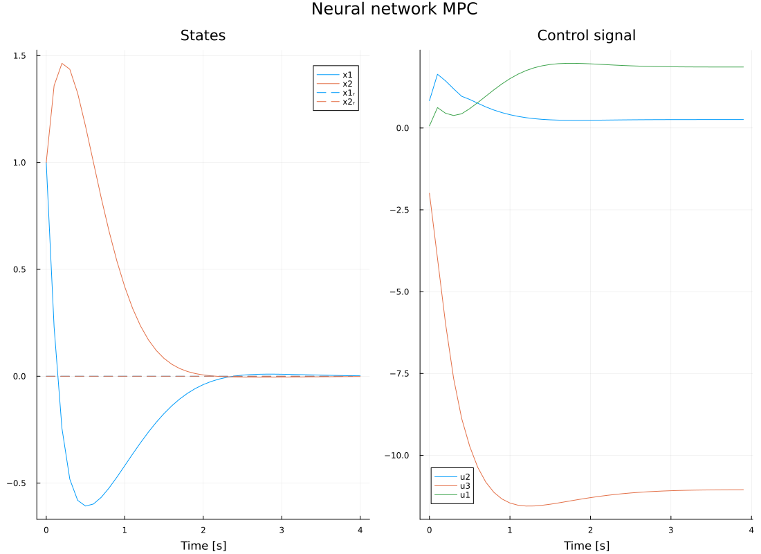
history = MPC.solve(prob; x0, T = 40, verbose = true); # Solve for 40 time steps

plot(history, plot_title="Neural network MPC")