Robust MPC with uncertain parameters

In this tutorial, we will construct an MPC controller that is robust with respect to uncertainty in one or several parameters of the system. The GenericMPCProblem supports explicit modeling of MPC problems with uncertain parameters, this can be used to perform optimization under uncertainty in order to guarantee constraint satisfaction despite the model uncertainty. The key steps required to implement a robust MPC controller are:

Construct a vector of possible parameter realizations. For example, if the gain of the system is uncertain, but known to be either 0.5, 1 or 5, then the vector of possible parameter realizations may be specified as $p = [1.0, 0.5, 5]$. We provide the nominal parameter realization first, i.e., the best guess of the parameter value and the parameter that the observer will be using.
Specify the robust_horizon over which the optimization problem forces control inputs to be identical for each instantiation of the uncertain plant.

In this example, we will control a simple linear system consisting of a single integrator only. We are going to implement two versions of the controller, the first one will use the nominal plant model only, $P(s) = 1/s$, while the second controller will use a model with explicit parameter uncertainty, $P(s) = k/s : \; k ∈ \left\{ 0.5, 1, 5\right\}$.

Nominal design

We start by defining the dynamics of the system:

using JuliaSimControl
using JuliaSimControl.MPC
using Plots, LinearAlgebra, StaticArrays

function linsys(x, u, p, _)
    A = SA[1.0;;]
    B = SA[p;;] # The gain depends on a parameter p = k
    A*x + B*u
end

Ts = 1          # Sample time
x0 = [10.0]     # Initial state
xr = [0.0]      # Reference state
dynamics = FunctionSystem(linsys, (x,u,p,t)->x, Ts, x=:x, u=:u, y=:y)

We then specify the cost function, in this case a simple quadratic state cost and a quadratic penalty on input differences. To make it extra interesting, we constrain the state to be $x \geq -0.5$ and the input to be $u \in [-4, 4]$ using a BoundsConstraint

running_cost = StageCost() do si, p, t
    e = si.x[] - si.r[]
    dot(e, e)
end
difference_cost = DifferenceCost() do e, p, t
    dot(e, e)
end
terminal_cost = TerminalCost() do ti, p, t
    e = ti.x[] - ti.r[]
    10dot(e, e)
end

bounds_constraint = BoundsConstraint(umin = [-4], umax = [4], xmin = [-0.5], xmax = [Inf])

objective = Objective(running_cost, terminal_cost, difference_cost)

We then specify the MPC horizon $N=10$, the nominal parameter $p=k=1$ and the MPC problem. Finally, we simulate the closed-loop system for $T=20$ time steps.

N = 10 # MPC horizon
observer = StateFeedback(dynamics, x0)

p = 1.0 # Nominal parameter k = 1
prob = GenericMPCProblem(
    dynamics;
    N,
    observer,
    objective,
    constraints = [bounds_constraint],
    p,
    xr,
    presolve = true,
)
hist = MPC.solve(prob; x0, T=20, verbose = false);
plot(hist, lab="Nominal MPC")

Robust design

The modification required to make this standard MPC controller robust w.r.t. variations of the gain is to specify a vector of possible parameter realizations, here, we call it p_uncertain. When making use of robust MPC, we must pass the parameters in the form of a vector of MPCParameters, this is to make sure that the MPC controller can distinguish between a set of uncertain parameters and a single parameter that is a vector. We then set the robust_horizon = 1 to indicate that we want to solve a robust MPC problem. The MPC controller will force the control input to be identical for each realization of the uncertain plant over the first robust_horizon samples. Usually, robust_horizon = 1 is sufficient to guarantee constraint satisfaction.^[1]

Finally, we solve the problem again and plot the results together with the nominal MPC controller.

p_uncertain = MPCParameters.([1.0; 0.5; 5]) # Place the nominal parameters first, k ∈ {1, 0.5, 5}
observer = StateFeedback(dynamics, x0)
probu = GenericMPCProblem(
    dynamics;
    N,
    observer,
    objective,
    constraints = [bounds_constraint],
    p = p_uncertain,
    xr,
    presolve = true,
    robust_horizon = 1,
);
histu = MPC.solve(probu; x0, T=20, verbose = false, p_actual=1.0);
plot!(histu, lab="Robust MPC", c=2)

As we can see, the robust controller is much more conservative with the input since the plant gain is highly uncertain.

To get a better feeling for how the robust optimization works, we can animate what the MPC controller thinks about the evolution of the system during the simulation. The code below creates a little animation where we plot the history using solid lines, and the future predictions according to each realization of the uncertain parameter as dashed lines.

anim = Plots.Animation()
function callback(actual_x, u, x, X, U)
    n_robust = length(p_uncertain)
    (; nx, nu) = dynamics
    T = length(X)
    tpast = 1:T
    fig = plot(
        tpast,
        reduce(hcat, X)',
        c       = (1:nx)',
        layout  = (nx+nu, 1),
        sp      = (1:nx)',
        ylabel  = "x",
        legend  = true,
        lab     = "History",
        xlims   = (1,25),
    )
    plot!(
        tpast,
        reduce(hcat, U)',
        c       = (1:nu)',
        sp      = (1:nu)' .+ nx,
        ylabel  = "u",
        legend  = true,
        lab     = "History",
        xlims   = (1,25),
    )

    xs = map(1:n_robust) do ri
        xu, uu = get_xu(probu, ri)
        xu
    end
    Xs = reduce(vcat, xs)
    tfuture = (1:size(Xs, 2)) .+ (T - 1)
    lab = permutedims(["Prediction \$k = \$ $(p_uncertain[i].p)" for i in 1:n_robust])
    plot!(tfuture, Xs'; c = (1:n_robust)', l = :dash, sp = (1:nx)', lab)

    us = map(1:n_robust) do ri
        xu, uu = get_xu(probu, ri)
        uu
    end
    Us = reduce(vcat, us)
    tfuture = (1:size(Us, 2)) .+ (T - 1)
    plot!(tfuture, Us'; c = (1:n_robust)', l = :dash, sp = (1:nu)'.+ nx, lab)
    hline!([bounds_constraint.xmin[1]], l = (:gray, :dash), lab = "Lower bound", sp=1)
    Plots.frame(anim, fig)
end

hist_anim = MPC.solve(probu; x0, T=15, p_actual=1.0, callback);
gif(anim, fps = 5)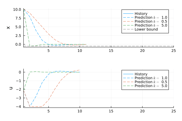

Here, we see that the MPC controller has three distinct predictions about the future, one for each instantiation of the uncertain plant gain $k$. We now clearly see why the robust controller is so conservative, this is required not ti overshoot the lower bound $x ≥ -0.1$ for the realization of the plant that has gain $k=10$. We also see that the controller optimizes three unique control-input trajectories, with the additional constraint that the first robust_horizon samples of the control input must be identical for all control-input trajectories. This approach has a number of nice properties

The controller avoids the excessive conservatism that would arise if a single control-input trajectory was optimized to control each uncertain realization. The controller predicts $N$ steps into the future, but after receiving new measurements, information about the actual realization of the plant is obtained, and the controller will thus be free to act differently after one sample depending on the actual realization of the uncertain plant. Another way to understand why the use of a single control-input trajectory would be conservative is that the controller optimizes an open-loop simulation of the uncertain plant, but the actual operation of the controller is in closed-loop, with new information arriving after time step.
The controller respects the fact that the first control input is taken with only the currently available information, and no new information about the uncertain plant is obtained until after one control input has been applied. Indeed, new information becomes available only after new measurements are received.

While optimizing, the MPC controller ensures constraint satisfaction for each realization of the uncertain plant, i.e., all the dashed lines in the animation are forced to obey the constraints. The cost function on the other hand is the sum over the uncertain realization of the plants, i.e., the sum of the costs for the trajectories represented by the dashed lines. This can be interpreted as a minimization of the expected cost if the set of uncertain parameters represents samples of a probability distribution of uncertain values.

The animation clearly indicates the uncertainty-suppressing properties of feedback. Despite the very large uncertainty in gain (10x), making the initial response highly uncertain (indicated by the spread of the first few samples of the dashed lines at each time step), the controller is able to reduce the variance of the response over the course of the optimization horizon due to feedback (indicated by low variance of the last few samples of the dashed lines at each time step).

Performance vs. robustness

The use of a robust controller comes at the cost of a performance penalty for the nominal case. We can quantify this tradeoff for this example by comparing the performance of the nominal controller designed for $k=1$, and robust controller, for different values of the uncertain parameter $k$. The code below simulates the nominal and robust controllers for different values of $k$, and plots the resulting trajectories.

fig = plot(layout=(3,2), grid=false, size=(700, 800))
figs = map(enumerate([0.5, 1.0, 5.0])) do (i, p_actual)
    hist = MPC.solve(prob; x0, T=20, verbose = false, p_actual=p_actual);
    histu = MPC.solve(probu; x0, T=20, verbose = false, p_actual=p_actual);
    plot!(hist, lab="Nominal", c=1, plotr=false, sp=(1:2)' .+ (i-1)*2)
    plot!(histu, lab="Robust", c=2, plotr=false, sp=(1:2)' .+ (i-1)*2, ylabel=["\$k\$ = $p_actual" ""], leftmargin=3Plots.mm)
    hline!([bounds_constraint.xmin[1]], l = (:gray, :dash), lab = "Lower bound", sp=1 + (i-1)*2)
end
fig

The figure indicates that while the robust controller has a significantly slower response when the gain is low or at the nominal value $k=1$, it behaves much better when the gain is higher than the nominal gain. When $k = 5$, the nominal controller even fails to satisfy the state constraint, while the possibility of $k$ being this large is taken into account by the robust controller.

Closing remarks

In this example, we implemented a robust MPC controller for a plant with a single uncertain parameter. We could let multiple parameters be uncertain by passing in a vector of composite data structures, e.g., a vector of vectors, where more than one parameter varies between each inner vector. We could also change the weighting of the different uncertain realizations in the cost function by passing parameters also to the cost functions. For example, the following definitions add weights to the cost functions and creates MPCParameters with separate parameters for the cost function that penalizes the nominal case with a weight of 1.0, and the other cases with a weight of 0.01.

running_cost = StageCost() do si, p, t
    e = p*(si.x-si.r)[1]
    dot(e, e)
end
difference_cost = DifferenceCost() do e, p, t
    p*dot(e, e)
end
terminal_cost = TerminalCost() do ti, p, t
    e = (ti.x-ti.r)[1]
    10p*dot(e, e)
end

p_uncertain = MPCParameters.([1.0; 0.5; 5], [1, 0.01, 0.01]) # Give a higher weight to the nominal case

See MPCParameters for more info.

Robust MPC with uncertain parameters

Nominal design

Robust design

Performance vs. robustness

Closing remarks

See also