Adaptive MPC

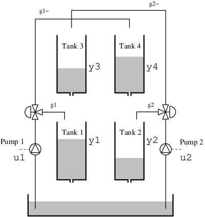
In this example, we will design a self-learning MPC controller that adapts to changes in the plant. We will consider a quadruple tank system with two inputs and two outputs, where the effectiveness of one pump is reduced in half halfway into the simulation.

This tutorial will use the QMPCProblem, a nonlinear MPC problem with quadratic cost function. We discretize the continuous-time dynamics using the rk4 function and set the prediction horizon for the MPC controller to N = 5.

We start by defining the dynamics and the MPC parameters, and use the parameter p to signal whether or not the change in the pump effectiveness is active or not. Since the problem is nonlinear, we use an UnscentedKalmanFilter for state estimation.

using JuliaSimControl
using JuliaSimControl.MPC
using Plots, LinearAlgebra
using StaticArrays
## Nonlinear quadtank
# p indicates whether or not k1 changes value at t = 1000
function quadtank(h, u, p, t)
    kc = 0.5
    k1, k2, g = 1.6, 1.6, 9.81
    A1 = A3 = A2 = A4 = 4.9
    a1, a3, a2, a4 = 0.03, 0.03, 0.03, 0.03
    γ1, γ2 = 0.3, 0.3
    if p == true && t > 1000
        k1 /= 2
    end

    ssqrt(x) = √(max(x, zero(x)) + 1e-3) # For numerical robustness at x = 0
    SA[
        -a1/A1 * ssqrt(2g*h[1]) + a3/A1*ssqrt(2g*h[3]) +     γ1*k1/A1 * u[1]
        -a2/A2 * ssqrt(2g*h[2]) + a4/A2*ssqrt(2g*h[4]) +     γ2*k2/A2 * u[2]
        -a3/A3*ssqrt(2g*h[3])                          + (1-γ2)*k2/A3 * u[2]
        -a4/A4*ssqrt(2g*h[4])                          + (1-γ1)*k1/A4 * u[1]
    ]
end

nu = 2 # number of control inputs
nx = 4 # number of state variables
ny = 2 # number of outputs
Ts = 1 # sample time

discrete_dynamics0 = rk4(quadtank, Ts) # Discretize the continuous-time dynamics
state_names = :h^4
measurement = (x,u,p,t) -> 0.5*x[1:2]
discrete_dynamics = FunctionSystem(discrete_dynamics0, measurement, Ts, x=state_names, u=:u^2, y=:h^2)


# Control limits
umin = 0 * ones(nu)
umax = 1 * ones(nu)

# State limits (state constraints are soft by default)
xmin = zeros(nx)
xmax = Float64[12, 12, 8, 8]
constraints = NonlinearMPCConstraints(; umin, umax, xmin, xmax)

x0 = [2, 1, 8, 3]       # Initial state
xr = [10, 10, 4.9, 4.9] # reference state
ur = [0.26, 0.26]

R1 = 1e-5*I(nx) # Dynamics covariance
R2 = 0.1I(ny)   # Measurement covariance

ukf = UnscentedKalmanFilter(discrete_dynamics, R1, R2)

solver = OSQPSolver(
    eps_rel = 1e-6,
    eps_abs = 1e-6,
    max_iter = 5000,
    check_termination = 5,
    sqp_iters = 1,
    dynamics_interval = 1,
    verbose = false,
    polish = true,
)

N  = 5          # MPC horizon
Q1 = 10I(nx)    # State cost
Q2 = 1.0*I(nu)  # Control cost
qs = 100        # Soft constraint linear penalty
qs2 = 100000    # Soft constraint quadratic penalty

prob = QMPCProblem(discrete_dynamics; observer=ukf, Q1, Q2, qs, qs2, constraints, N, xr, ur, solver, p=false)

QMPCProblem{FunctionSystem{Discrete{Int64}, SeeToDee.Rk4{typeof(Main.quadtank), Float64}, Main.var"#2#3", Vector{Symbol}, Vector{Symbol}, Vector{Symbol}, Nothing, UnitRange{Int64}, SciMLBase.NullParameters, UnitRange{Int64}, Nothing}, UnscentedKalmanFilter{SeeToDee.Rk4{typeof(Main.quadtank), Float64}, Main.var"#2#3", LinearAlgebra.Diagonal{Float64, Vector{Float64}}, LinearAlgebra.Diagonal{Float64, Vector{Float64}}, Distributions.ZeroMeanFullNormal{Tuple{Base.OneTo{Int64}}}, StaticArraysCore.SVector{4, Float64}, Vector{Float64}, Matrix{Float64}, SciMLBase.NullParameters}, Vector{Float64}, Matrix{Int64}, LinearAlgebra.Diagonal{Float64, Vector{Float64}}, SparseArrays.SparseMatrixCSC{Float64, Int64}, NonlinearMPCConstraints{JuliaSimControl.MPC.var"#28#30"{SparseArrays.SparseMatrixCSC{Float64, Int64}, SparseArrays.SparseMatrixCSC{Float64, Int64}}, Vector{Float64}, UnitRange{Int64}}, Vector{Float64}, SparseArrays.SparseMatrixCSC{Float64, Int64}, Vector{CartesianIndex{2}}, JuliaSimControl.MPC.OSQPSolverWorkspace, ForwardDiff.Chunk{4}, ForwardDiff.Chunk{2}, Matrix{Float64}, Bool}(FunctionSystem{Discrete{Int64}, SeeToDee.Rk4{typeof(Main.quadtank), Float64}, Main.var"#2#3", Vector{Symbol}, Vector{Symbol}, Vector{Symbol}, Nothing, UnitRange{Int64}, SciMLBase.NullParameters, UnitRange{Int64}, Nothing}(SeeToDee.Rk4{typeof(Main.quadtank), Float64}(Main.quadtank, 1.0, 1), Main.var"#2#3"(), Discrete{Int64}(1), [:h1, :h2, :h3, :h4], [:u1, :u2], [:h1, :h2], nothing, 1:4, SciMLBase.NullParameters(), 0:-1, nothing), UnscentedKalmanFilter{SeeToDee.Rk4{typeof(Main.quadtank), Float64}, Main.var"#2#3", LinearAlgebra.Diagonal{Float64, Vector{Float64}}, LinearAlgebra.Diagonal{Float64, Vector{Float64}}, Distributions.ZeroMeanFullNormal{Tuple{Base.OneTo{Int64}}}, StaticArraysCore.SVector{4, Float64}, Vector{Float64}, Matrix{Float64}, SciMLBase.NullParameters}
  dynamics: SeeToDee.Rk4{typeof(Main.quadtank), Float64}
  measurement: #2 (function of type Main.var"#2#3")
  R1: LinearAlgebra.Diagonal{Float64, Vector{Float64}}
  R2: LinearAlgebra.Diagonal{Float64, Vector{Float64}}
  d0: Distributions.ZeroMeanFullNormal{Tuple{Base.OneTo{Int64}}}
  xs: Array{StaticArraysCore.SVector{4, Float64}}((9,))
  x: Array{Float64}((4,)) [0.0, 0.0, 0.0, 0.0]
  R: Array{Float64}((4, 4)) [1.0e-5 0.0 0.0 0.0; 0.0 1.0e-5 0.0 0.0; 0.0 0.0 1.0e-5 0.0; 0.0 0.0 0.0 1.0e-5]
  t: Base.RefValue{Int64}
  ny: Int64 2
  nu: Int64 2
  p: SciMLBase.NullParameters SciMLBase.NullParameters()
, [10.0, 10.0, 4.9, 4.9], [0.26, 0.26], [10 0 0 0; 0 10 0 0; 0 0 10 0; 0 0 0 10], [1.0 0.0; 0.0 1.0], nothing, sparse([1, 2, 3, 4, 1, 2, 3, 4, 1, 2, 3, 4, 1, 2, 3, 4], [1, 1, 1, 1, 2, 2, 2, 2, 3, 3, 3, 3, 4, 4, 4, 4], [844.6162600230527, -295.8348831561848, 133.41667055969367, -355.604496181032, -295.8348831561848, 844.6162600219434, -355.6044961805568, 133.41667055968452, 133.41667055969367, -355.6044961805568, 171.70470301044494, -59.9843047178875, -355.604496181032, 133.41667055968452, -59.9843047178875, 171.7047030106484], 4, 4), 100.0, 100000.0, NonlinearMPCConstraints{JuliaSimControl.MPC.var"#28#30"{SparseArrays.SparseMatrixCSC{Float64, Int64}, SparseArrays.SparseMatrixCSC{Float64, Int64}}, Vector{Float64}, UnitRange{Int64}}(JuliaSimControl.MPC.var"#28#30"{SparseArrays.SparseMatrixCSC{Float64, Int64}, SparseArrays.SparseMatrixCSC{Float64, Int64}}(sparse([5, 6], [1, 2], [1.0, 1.0], 6, 2), sparse([1, 2, 3, 4], [1, 2, 3, 4], [1.0, 1.0, 1.0, 1.0], 6, 4)), [0.0, 0.0, 0.0, 0.0, 0.0, 0.0], [12.0, 12.0, 8.0, 8.0, 1.0, 1.0], 1:4), 5, sparse([1, 2, 3, 4, 5, 6, 7, 8, 9, 10  …  73, 74, 71, 72, 73, 74, 71, 72, 73, 74], [1, 2, 3, 4, 5, 6, 7, 8, 9, 10  …  72, 72, 73, 73, 73, 73, 74, 74, 74, 74], [10.0, 10.0, 10.0, 10.0, 1.0, 1.0, 100000.0, 100000.0, 100000.0, 100000.0  …  -355.6044961805568, 133.41667055968452, 133.41667055969367, -355.6044961805568, 171.70470301044494, -59.9843047178875, -355.604496181032, 133.41667055968452, -59.9843047178875, 171.7047030106484], 74, 74), [-100.0, -100.0, -49.0, -49.0, 0.0, 0.0, 100.0, 100.0, 100.0, 100.0  …  100.0, 100.0, 100.0, 100.0, 100.0, 100.0, -4399.093423124121, -4399.093423115311, 1674.4483045751, 1674.448304578947], sparse([1, 5, 25, 31, 2, 6, 26, 32, 3, 5  …  80, 122, 81, 123, 82, 124, 21, 22, 23, 24], [1, 1, 1, 1, 2, 2, 2, 2, 3, 3  …  68, 68, 69, 69, 70, 70, 71, 72, 73, 74], [-1.0, 0.9957212628605769, 1.0, 1.0, -1.0, 0.9957212628605769, 1.0, 1.0, -1.0, 0.006093916176921524  …  1.0, 1.0, 1.0, 1.0, 1.0, 1.0, -1.0, -1.0, -1.0, -1.0], 124, 74), [-0.0, -0.0, -0.0, -0.0, 0.0, 0.0, 0.0, 0.0, 0.0, 0.0  …  0.0, 0.0, 0.0, 0.0, 0.0, 0.0, 0.0, 0.0, 0.0, 0.0], [-0.0, -0.0, -0.0, -0.0, 0.0, 0.0, 0.0, 0.0, 0.0, 0.0  …  Inf, Inf, Inf, Inf, Inf, Inf, Inf, Inf, Inf, Inf], CartesianIndex{2}[CartesianIndex(1, 1), CartesianIndex(2, 2), CartesianIndex(1, 3), CartesianIndex(3, 3), CartesianIndex(2, 4), CartesianIndex(4, 4)], CartesianIndex{2}[CartesianIndex(1, 1), CartesianIndex(2, 1), CartesianIndex(4, 1), CartesianIndex(1, 2), CartesianIndex(2, 2), CartesianIndex(3, 2)], JuliaSimControl.MPC.OSQPSolverWorkspace(OSQP.Model(Ptr{OSQP.Workspace} @0x000000000776ae30, [6.9494860641447e-310, 5.93e-322, 2.782597e-318, 5.93e-322, 5.93e-322, 6.9494707338138e-310, 6.9494707338209e-310, 6.94947073382327e-310, 6.94947073382564e-310, 6.949470733828e-310  …  6.9494707340865e-310, 6.9494707340889e-310, 6.94947073409125e-310, 6.94947073409363e-310, 6.949470734096e-310, 6.9494707341126e-310, 6.94947073411497e-310, 6.94947073411734e-310, 6.9494707341197e-310, 6.9494707341221e-310], [5.0e-324, 0.0, 5.0e-324, 1.5e-323, 5.0e-324, 6.94945879695305e-310, 2.5e-323, 1.3e-322, 6.94948326529725e-310, 2.0e-323  …  6.949485714115e-310, 6.9494857141134e-310, 6.94971745568207e-310, 0.0, 6.94971745568207e-310, 0.0, 1.83e-322, 1.43e-322, 5.0e-324, 6.94948231888955e-310], false), OSQPSolver(false, 1.0e-6, 1.0e-6, 5000, 5, 1, 1, true, 1.0e10)), ForwardDiff.Chunk{4}(), ForwardDiff.Chunk{2}(), [0.0 0.0 … 0.0 0.0; 0.0 0.0 … 0.0 0.0; 0.0 0.0 … 0.0 0.0; 0.0 0.0 … 0.0 0.0], [0.0 0.0 … 0.0 0.0; 0.0 0.0 … 0.0 0.0], false, 4, [0.0 0.0 … 0.0 0.0; 0.0 0.0 … 0.0 0.0; … ; 0.0 0.0 … 0.0 0.0; 0.0 0.0 … 0.0 0.0])

When we solve the problem, the prediction model uses p=false, i.e., it's not aware of the change in dynamics, but the actual dynamics has p=true so the simulated system will suffer from the change

hist = MPC.solve(prob; x0, T = 2000, verbose = false, dyn_actual=discrete_dynamics, p=false, p_actual=true)
plot(hist, plot_title="Standard Nonlinear MPC")

At $t = 1000$ we see that the states drift away from the references and the controller does little to compensate for it. Let's see if an adaptive MPC controller can improve upon this!

To make the controller adaptive, we introduce an additional state in the dynamics. When the observer estimates the state of the system, it will automatically estimate the value of this parameter, and this state will thus serve to estimate the pump effectiveness, and takes the place of the k1 parameter from before. If we have no idea exactly how the change will happen, we could say that the derivative of the unknown parameter is 0, and thus model a situation in which this state is driven by noise only. We'll take this route, but will make the dynamics of the unknown state ever so slightly stable for numerical purposes.

function quadtank_param(h, u, p, t)
    k2, g = 1.6, 9.81
    A1 = A3 = A2 = A4 = 4.9
    a1, a3, a2, a4 = 0.03, 0.03, 0.03, 0.03
    γ1, γ2 = 0.3, 0.3

    k1 = h[5]

    ssqrt(x) = √(max(x, zero(x)) + 1e-3) # For numerical robustness at x = 0
    SA[
        -a1/A1 * ssqrt(2g*h[1]) + a3/A1*ssqrt(2g*h[3]) +     γ1*k1/A1 * u[1]
        -a2/A2 * ssqrt(2g*h[2]) + a4/A2*ssqrt(2g*h[4]) +     γ2*k2/A2 * u[2]
        -a3/A3*ssqrt(2g*h[3])                          + (1-γ2)*k2/A3 * u[2]
        -a4/A4*ssqrt(2g*h[4])                          + (1-γ1)*k1/A4 * u[1]
        1e-4*(1.6 - k1) # The parameter state is not controllable, we thus make it ever so slightly exponentially stable to ensure that the Riccati solver can find a solution.
    ]
end
state_names = [:h^4; :k1]
discrete_dynamics_param = FunctionSystem(rk4(quadtank_param, Ts), measurement, Ts, x=state_names, u=:u^2, y=:h^2)
nx = 5 # number of state variables, one more this time due to the parameter state

xmin = 0 * ones(nx)
xmax = Float64[12, 12, 8, 8, 100]
constraints = NonlinearMPCConstraints(; umin, umax, xmin, xmax)

x0 = [2, 1, 8, 3, 1.6]       # Initial state
xr = [10, 10, 4.9, 4.9, 1.6] # reference state, provide a good guess for the uncertain parameter since this point determins linearization.
ur = [0.26, 0.26]

R1 = cat(1e-5*I(nx-1), 1e-5, dims=(1,2)) # Dynamics covariance

ukf = UnscentedKalmanFilter(
    discrete_dynamics_param.dynamics,
    discrete_dynamics_param.measurement,
    R1,
    R2,
    MvNormal(x0, Matrix(R1))
    ;
    nu,
    ny
)
#
Q1 = cat(10I(nx-1), 0, dims=(1,2)) # We do not penalize the parameter state, it is not controllable
prob = QMPCProblem(discrete_dynamics_param; observer=ukf, Q1, Q2, qs, qs2, constraints, N, xr, ur, solver, p=true)
hist = MPC.solve(prob; x0, T = 2000, verbose = false, dyn_actual=discrete_dynamics, x0_actual = x0[1:nx-1], p=false, p_actual=true)
plot(hist, plot_title="Adaptive Nonlinear MPC")

This time, the simulation looks much better and the controller quickly recovers after the change in dynamics at $t = 1000$.

We can check what value of the estimated parameter the state estimator converged to

using Test
@test ukf.x[5] ≈ 0.8 atol=0.02

Test Passed

which should be close to $1.6 / 2 = 0.8$ if the observer has worked correctly.