Tuning objectives
When designing a control system, it is common to work towards satisfying a number requirements. In DyadControlSystems, such requirements can be encoded in TuningObjectives, an abstract type that affords both visualization and optimization controllers to meet tuning requirements. The objectives can thus be used for two primary tasks
- Visualization of requirements
- Optimization-based autotuning
which we cover in the following sections:
The first section below indicates how to construct tuning objectives and visualize them in a plot, while the subsequent section demonstrates their usage for automatic controller tuning in a ModelingToolkit model. This tutorial is available also in video form:
Visualize performance and robustness requirements
We illustrate how performance and robustness specifications can be visualized by creating instances of objective types for which plot recipes are available.
using DyadControlSystems, Plots
G = tf(2, [1, 0.3, 2])           # An example system
w = exp10.(LinRange(-2, 2, 200)) # A frequency vector

W = tf([2, 0], [1, 1]) # A weight specifying the maximum allowed sensitivity
S = feedback(1, G)     # The sensitivity function
bodeplot(S, w, plotphase=false)
plot!(MaximumSensitivityObjective(W), w, title="MaximumSensitivityObjective")
plot(step(G, 15))
plot!(OvershootObjective(1.2), title="OvershootObjective")
plot(step(G, 15))
plot!(RiseTimeObjective(0.6, 1), title="RiseTimeObjective")
plot(step(G, 15))
plot!(SettlingTimeObjective(1, 5, 0.2), title="SettlingTimeObjective")
plot(step(G, 15))
o = StepTrackingObjective(tf(1, [1,2,1])) # Takes a reference model
plot!(o, title="StepTrackingObjective")
StepTrackingObjective for step rejection:
plot(step(G*feedback(1, G), 15))
o = StepTrackingObjective(tf([1, 0], [1,2,1])) # Takes a reference model
plot!(o, title="Step rejection using StepTrackingObjective")
GainMarginObjective and PhaseMarginObjective:
dm = diskmargin(G, 0, w)
plot(dm)
plot!(GainMarginObjective(2),   title="GainMarginObjective")
plot!(PhaseMarginObjective(45), title="PhaseMarginObjective")
Automatic tuning of structured controllers
In this section, we will explore how we can make use of the tuning objectives illustrated above for automatic tuning of structured controllers. Each tuning objective can upon creation take one or several signals that relate to a model in which we want to tune the control performance. This functionality is built around the concept of an analysis point, which for the purposes of autotuning can be thought of as a named signal of interest in the model. Analysis points can be used to linearize the model and compute sensitivity functions automatically, something that is required for the autotuning functionality.
We demonstrate the usage by means of a simple example, where we first perform tuning of a PI speed controller for a DC motor, and then add an outer position-control loop to form a cascade control architecture, where both loops are automatically tuned.
Example: PI controller tuning for a DC motor
The system to control is a DC motor with a PI controller for the velocity. See the DC-motor tutorial for how to build this system, insert analysis points and compute sensitivity functions. In the present tutorial, we will load the pre-built system from DyadControlSystems.ControlDemoSystems.dcmotor(). This system contains three analysis points, r, u, y for the reference, control signal and output of the velocity sensor.
The block diagram below shows a typical control architecture for a motion-control system, which is the final system we will work towards. In this section, we are currently concerned with tuning $K_v$ and $K_i$, the proportional and integral gains for a PI velocity controller. The outer loop closed through $K_p$ will be added in the next section. 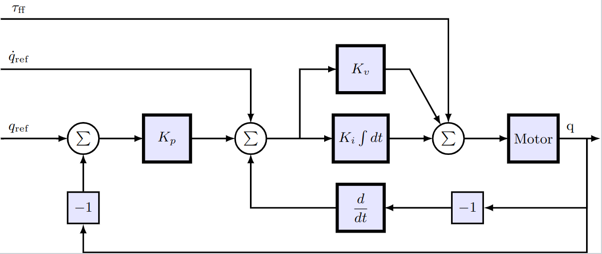
using DyadControlSystems, DyadControlSystems.MPC
using ModelingToolkit

sys = DyadControlSystems.ControlDemoSystems.dcmotor()
We then specify the parameters we want to tune as a vector of pairs, from parameter to a tuple of bounds. In this case, we tune the proportional gain and the gain of the integrator in the controller. To be able to refer to the parameters correctly, we call complete on the model first. We also specify one or several operating points in which we want to tune the parameters. This system is linear, so a single operating point is sufficient. Had the system been nonlinear, or some parameters of the system were uncertain, we could specify several points here and the tuning would be done to meet requirements for all operating points. An operating point is here defined as a dictionary of variable => value pairs, where the variables include both states and parameters for the system. In this case, we use the defaults already defined in the system.
sysc = complete(sys)
tunable_parameters = [
    sysc.pi_controller.gainPI.k => (1e-9, 100.0) # parameter => (lower_bound, upper_bound)
    sysc.pi_controller.int.k    => (2.0, 1e2)
]

operating_points = [ # Can be one or several operating points
    Dict(sysc.L1.p.i => 0.0)
]An operating point is typically understood as a tuple of the form $(x, u)$, where $x$ is the state vector and $u$ is the input vector. However, we may choose to include parameters $p$ in the operating point as well. This may be useful when some parameters are uncertain or time varying, and we want to perform analysis over multiple possible parameter values.
The next step is to define our requirements by specifying tuning objectives. We will include 4 objectives for the purpose of demonstration, but it is often sufficient to use a smaller number of objectives. Note, however, that it is often best to include at least one performance promoting objective and one robustness promoting objective.
The StepTrackingObjective allows us to specify a reference model ($G_{ref}$) that indicates how we want a step-response of the closed-loop system to behave. In this case, we consider the step response from analysis point r to y. We also include a constraint on the sensitivity function at the plant output y, with a weight $W_S$. These two objectives are often a good start, but here we add also a OvershootObjective and a RiseTimeObjective to fine-tune the transient response and demonstrate their usage.
WS    = tf([1.5, 0], [1, 50])
ω     = 2pi*20.0
Gref  = tf(ω^2, [1, 2ω, ω^2])
sto   = StepTrackingObjective(reference_model=Gref, tolerance=0.05, input=sys.r, output=sys.y)
mso   = MaximumSensitivityObjective(WS, sys.y)
oo    = OvershootObjective(max_value = 1.05, input=sys.r, output=sys.y)
rto   = RiseTimeObjective(min_value = 0.91, time = 0.025, input=sys.r, output=sys.y)
seto  = SettlingTimeObjective(; final_value = 1.0, time = 0.025, tolerance = 0.09, input=sys.r, output=sys.y) # We do not use this objective here, but one sometimes trades the overshoot and rise-time objectives for this objective
objectives = [
    sto,
    mso,
    oo,
    rto,
    # seto,
]
4-element Vector{DyadControlSystems.TuningObjective}:
Step tracking dcmotor₊r → dcmotor₊y with tol 0.05
Max sensitivity at dcmotor₊y
Overshoot dcmotor₊r → dcmotor₊y ≤ 1.05
Rise time dcmotor₊r → dcmotor₊y ≥ 0.91 after t=0.025The last step before defining the problem is to specify time and frequency grids at which to evaluate the objectives. Denser grids make the result more accurate, but increases the time to solution.
w = exp10.(LinRange(0, 3, 200))
t = 0:0.001:0.21
We now define the problem:
prob = StructuredAutoTuningProblem(sys, w, t, objectives, operating_points, tunable_parameters)StructuredAutoTuningProblem
sys : dcmotor
num frequencies : 200 between 1 and 1e+03
num time points : 211 between 0 and 0.21
num operating points: 1
objectives :
Step tracking dcmotor₊r → dcmotor₊y with tol 0.05
Max sensitivity at dcmotor₊y
Overshoot dcmotor₊r → dcmotor₊y ≤ 1.05
Rise time dcmotor₊r → dcmotor₊y ≥ 0.91 after t=0.025
tunable parameters :
pi_controller₊gainPI₊k => (1.0e-9, 100.0)
pi_controller₊int₊k => (2.0, 100.0)
To solve it, we specify an initial guess for the parameters, this is a vector in the same order as the tunable_parameters. The solver can be chosen freely among the solvers that are supported in Optimization.jl
p0 = [1.0, 20] # Initial guess
res = solve(prob, p0,
    MPC.IpoptSolver(verbose=true, exact_hessian=false, acceptable_iter=4, tol=1e-3, acceptable_tol=1e-2, max_iter=100);
)
StructuredAutoTuningResult
sys : dcmotor
num frequencies : 200 between 1 and 1e+03
num time points : 211 between 0 and 0.21
num operating points: 1
objectives
Step tracking dcmotor₊r → dcmotor₊y with tol 0.05
Max sensitivity at dcmotor₊y
Overshoot dcmotor₊r → dcmotor₊y ≤ 1.05
Rise time dcmotor₊r → dcmotor₊y ≥ 0.91 after t=0.025
tunable parameters
pi_controller₊gainPI₊k => (1.0e-9, 100.0)
pi_controller₊int₊k => (2.0, 100.0)
optimization status : MaxIters
objective status
:StepTrackingObjective => 0.11821298651236407
:MaximumSensitivityObjective => 0.005422241090663804
:OvershootObjective => 0.0
:RiseTimeObjective => 0.008649205435778344
minimizer
pi_controller₊gainPI₊k => 1.4354073402584793
pi_controller₊int₊k => 15.828874908338078
objective value : 1.616894730967632
When the problem has been solved, we may plot the results
plot(res)
This shows one plot for each tuning objective. In this case, we approximately meet all the requirement, save for the rise-time requirement that shows a slight violation. In general, it may not be feasible to meet all requirements, and the result will be a trade-off between them all. The field res.objective_status contains diagnostics for each operating point, where each entry indicates the relative satisfaction of each tuning objective, smaller values are better.
res.objective_status[1] # Inspect the results in the first (and in this case only) operating point4-element Vector{Pair{Symbol, Float64}}:
:StepTrackingObjective => 0.11821298651236407
:MaximumSensitivityObjective => 0.005422241090663804
:OvershootObjective => 0.0
:RiseTimeObjective => 0.008649205435778344Adding an outer position loop
In the example thus far, we have closed the velocity loop using PI controller. As mentioned above, a common control architecture for position-controlled systems is to add an outer P controller that controls the position, forming a cascade controller. In this section, we will add such an outer position loop, $K_p$ in the block diagram, and tune both controllers automatically. This time, we create the DC-motor system using dcmotor(ref=nothing) to indicate that we want nothing connected to the reference of the inner PI controller, and we add new connections corresponding to the outer loop. The P controller for the position loop uses a Blocks.Gain() block. To get good performance, it's important to add a velocity feedforward connection directly to the velocity controller, $\dot{q}_{ref}$ in the block diagram, without this, the velocity loop would be error driven only, necessitating an error for the system to move (more comments on this in the next section).
sys_inner             = DyadControlSystems.ControlDemoSystems.dcmotor(ref=nothing)
@named ref            = Blocks.Step(height = 1, start_time = 0)
@named ref_diff       = Blocks.Derivative(T=0.1) # This will differentiate q_ref to q̇_ref
@named add            = Blocks.Add()      # The middle ∑ block in the diagram
@named p_controller   = Blocks.Gain(10.0) # Kₚ
@named outer_feedback = Blocks.Feedback() # The leftmost ∑ block in the diagram
@named id             = Blocks.Gain(1.0)  # a trivial identity element to allow us to place the analysis point :r in the right spot

connect = ModelingToolkit.connect
connections = [
    connect(ref.output, :r, id.input)                               # We now place analysis point :r here
    connect(id.output, outer_feedback.input1, ref_diff.input)
    connect(ref_diff.output, add.input1)
    connect(add.output, sys_inner.feedback.input1)
    connect(p_controller.output, :up, add.input2)                   # Analysis point :up
    connect(sys_inner.angle_sensor.phi, :yp, outer_feedback.input2) # Analysis point :yp
    connect(outer_feedback.output, :ep, p_controller.input)         # Analysis point :ep
]

@named closed_loop = System(connections, ModelingToolkit.get_iv(sys_inner); systems = [sys_inner, ref, id, ref_diff, add, p_controller, outer_feedback])
We will use a MaximumSensitivityObjective for the inner loop, since this loop is primarily concerned with rejecting disturbances. When creating this objective, we specify loop_openings=[:yp] to indicate that we want to compute the sensitivity function at the velocity output with the position loop :yp opened (more info about this in the section below).
cl = complete(closed_loop)

tunable_parameters = [
    cl.dcmotor.pi_controller.gainPI.k => (1e-1, 10.0)
    cl.dcmotor.pi_controller.int.k    => (2.0, 1e2)
    cl.p_controller.k                 => (1e-2, 1e2)
]

operating_points = [ # Can be one or several operating points
    Dict(cl.dcmotor.L1.p.i => 0.0)
]

ωp    = 2pi*3.0                     # Desired position-loop bandwidth
Pref  = tf(ωp^2, [1, 2ωp, ωp^2])    # Desired position step response
stp   = StepTrackingObjective(reference_model = Pref, tolerance = 0.05, input=closed_loop.r, output=closed_loop.yp)
mso2  = MaximumSensitivityObjective(weight=WS, output=closed_loop.dcmotor.y, loop_openings=[closed_loop.yp])
objectives = [
    stp,
    mso2,
]

w = exp10.(LinRange(0, 3, 200))
t = 0:0.001:1
prob = DyadControlSystems.StructuredAutoTuningProblem(closed_loop, w, t, objectives, operating_points, tunable_parameters)

x0 = [1.0, 20, 0.1]
res = solve(prob, x0,
    MPC.IpoptSolver(verbose=true, exact_hessian=false, acceptable_iter=4, tol=1e-3, acceptable_tol=1e-2, max_iter=100);
)
StructuredAutoTuningResult
sys : closed_loop
num frequencies : 200 between 1 and 1e+03
num time points : 1001 between 0 and 1
num operating points: 1
objectives
Step tracking closed_loop₊r → closed_loop₊yp with tol 0.05
Max sens at closed_loop₊dcmotor₊y with openings [:closed_loop₊yp]
tunable parameters
dcmotor₊pi_controller₊gainPI₊k => (0.1, 10.0)
dcmotor₊pi_controller₊int₊k => (2.0, 100.0)
p_controller₊k => (0.01, 100.0)
optimization status : Success
objective status
:StepTrackingObjective => 0.11588293859527454
:MaximumSensitivityObjective => 0.0
minimizer
dcmotor₊pi_controller₊gainPI₊k => 1.1519285235463679
dcmotor₊pi_controller₊int₊k => 20.031210703375812
p_controller₊k => 0.08101285783706856
objective value : 0.11618279155212971
plot(res)
We can simulate the nonlinear system with the optimized operating point
using OrdinaryDiffEq
ssys = mtkcompile(closed_loop)
optimal_op = res.op[1]
optimal_op[ssys.dcmotor.L1.n.i] = 0.0
simprob = ODEProblem(ssys, optimal_op, (0.0, 1.0))
sol = solve(simprob, Tsit5())
plot(sol, idxs=[ssys.dcmotor.inertia.phi, ssys.ref.output.u])
A note about the loop opening
Why did we open the position loop when we computed the sensitivity function at the velocity output? The position loop fundamentally changes the closed-loop behavior of the system, compare the sensitivity functions below, computed with and without the loop closed
op1 = res.op[1]
wsens = exp10.(LinRange(-2, 3, 200))
bodeplot([
    ss(get_sensitivity(closed_loop, closed_loop.dcmotor.y; op=op1)[1]...),
    ss(get_sensitivity(closed_loop, closed_loop.dcmotor.y; op=op1, loop_openings=[closed_loop.yp])[1]...)
    ], wsens, plotphase = false,
    lab    = ["Position loop closed" "Position loop open"],
    title  = "Sensitivity at velocity output", size=(500, 300),
    legend = :bottomright
)
The output sensitivity function is the transfer function from the reference to the control error, and without the position loop, the velocity controller is able to track low-frequency velocity references perfectly due to the integrator in the PI controller. When we add the outer position loop, we are no longer free to set the velocity to whatever we want, and it's instead the position controller that dictates the reference for the velocity controller, this manifests itself as an inability to follow independent velocity references for low frequencies.
Had we not included the velocity feedforward from the reference to the velocity controller, we would instead have obtained the following result
op_no_vel_ff = deepcopy(res.op[1])
op_no_vel_ff[ref_diff.k] = 0 # Turn off velocity feedforward
prob2 = DyadControlSystems.StructuredAutoTuningProblem(closed_loop, w, t, objectives, [op_no_vel_ff], tunable_parameters)

res2 = solve(prob2, x0,
    MPC.IpoptSolver(verbose=true, exact_hessian=false, acceptable_iter=4, tol=1e-3, acceptable_tol=1e-2, max_iter=100);
)
plot(res2)
with the following sensitivity function
op_no_vel_ff = res2.op[1]
bodeplot([
    ss(get_sensitivity(closed_loop, closed_loop.dcmotor.y; op=op_no_vel_ff)[1]...),
    ss(get_sensitivity(closed_loop, closed_loop.dcmotor.y; op=op_no_vel_ff, loop_openings=[closed_loop.yp])[1]...)
    ], wsens, plotphase = false,
    lab    = ["Position loop closed" "Position loop open"],
    title  = "Sensitivity without velocity feedforward", size=(500, 300),
    legend = :bottomright
)
i.e., while the controller still appears to track the reference step quite well, the sensitivity function at the velocity output looks significantly worse, indicating that the closed-loop system will suffer quite poor disturbance-rejection properties, and likely be sensitive to model errors.
Tuning with uncertain parameters
The autotuning framework supports modeling and solving autotuning problems with parametric uncertainty, something we will explore in this section. Uncertainty is the fundamental reason we are making use of feedback, and parametric uncertainty is a particularly intuitive form of uncertainty that is easy to reason about. When tuning a controller, we may want to model known parametric uncertainty and make sure the tuned closed-loop system is robust with respect to known parameter variations.
Below, we solve the same autotuning problem as in the example where we tuned the PI velocity controller above, but in this case we model a uniformly distributed uncertainty in the inertia of the rotating load. To tell the system that a particular parameter is uncertain, give it an uncertain value in the form of MonteCarloMeasurements.Particles. Below, we construct a uniformly sampled uncertain value between 0.015 and 0.025 with N = 5 samples like so: Particles(N, Uniform(0.015, 0.025)). We may choose any distribution of our choice, but if we have more than one uncertain parameter, they must all use the same number of samples N.
using MonteCarloMeasurements
N = 5 # Number of samples for the uncertain parameters
sys = DyadControlSystems.ControlDemoSystems.dcmotor()
sysc = complete(sys)
op = Dict()
op[sysc.inertia.J] = Particles(N, Uniform(0.015, 0.025))
op[sysc.L1.p.i] = 0.0
operating_points = [op]
1-element Vector{Dict{Any, Any}}:
Dict(inertia₊J => 0.02 ± 0.0032, L1₊p₊i(t) => 0.0)Otherwise we proceed exactly like before:
tunable_parameters = [
    sysc.pi_controller.gainPI.k => (1e-9, 100.0)
    sysc.pi_controller.int.k    => (2.0, 1e2)
]

objectives = [
    sto,
    seto,
    mso,
]

w = exp10.(LinRange(0, 3, 200))
t = 0:0.001:0.21
prob = StructuredAutoTuningProblem(sys, w, t, objectives, operating_points, tunable_parameters)

x0 = [1.0, 20]
res = solve(prob, x0,
    MPC.IpoptSolver(verbose=true, exact_hessian=false, acceptable_iter=4, tol=1e-3, acceptable_tol=1e-2, max_iter=100);
)

plot(res)
This time, we see that the optimized controller is unable to satisfy all requirements for all instantiations of the uncertain system, maybe we're asking too much from a simple PID controller?[1]
Underneath the hood, the uncertain operating point is expanded into N = 5 operating points, and the optimizer tries to satisfy the tuning requirements for all of them. If we had used more than one operating point in the vector operating_points, we would get a total of N*length(operating_points) total operating points in the optimization problem.
Index
DyadControlSystems.GainMarginObjectiveDyadControlSystems.MaximumSensitivityObjectiveDyadControlSystems.MaximumTransferObjectiveDyadControlSystems.OvershootObjectiveDyadControlSystems.PhaseMarginObjectiveDyadControlSystems.RiseTimeObjectiveDyadControlSystems.SettlingTimeObjectiveDyadControlSystems.SimulationObjectiveDyadControlSystems.StepTrackingObjectiveDyadControlSystems.StructuredAutoTuningProblemDyadControlSystems.StructuredAutoTuningResultCommonSolve.solve
CommonSolve.solve — Function
solve(
    prob::StructuredAutoTuningProblem,
    x0,
    alg = MPC.IpoptSolver(
        verbose         = true,
        exact_hessian   = false,
        acceptable_iter = 4,
        tol             = 1e-3,
        acceptable_tol  = 1e-2,
        max_iter        = 100,
    );
    verbose = true,
    kwargs...,
)
Solve a structured parametric autotuning problem. The result can be plotted with plot(result).
Arguments:
prob: An instance of StructuredAutoTuningProblem holding tunable parameters and tuning objectives.x0: A vector of initial guesses for the tunable parameters, in the same order asprob.tunable_parameters.alg: An optimization algorithm compatible with Optimization.jl.verbose: Print diagnostic information?kwargs: Are passed tosolveon the optimization problem from Optimization.jl.
DyadControlSystems.GainMarginObjective — Type
GainMarginObjective(; margin, output, loop_openings)A tuning objective that lower bounds the gain margin of the system.
Fields:
margin: The desired margin in absolute scale, i.e. formargin = 2, the closed-loop is robust w.r.t. gain variations within a factor of two.output: The signal to compute the gain margin in.loop_openings: A list of analysis points in which the loop will be opened before computing the objective. See MTK stdlib: Linear analysis for more info on loop openings.
DyadControlSystems.MaximumSensitivityObjective — Type
MaximumSensitivityObjective(; weight, output, loop_openings)A tuning objective that upper bounds the sensitivity function at the signal output.
The output sensitivity function $S_o = (I + PC)^{-1}$ is the transfer function from a reference input to control error, while the input sensitivity function $S_i = (I + CP)^{-1}$ is the transfer function from a disturbance at the plant input to the total plant input. For SISO systems, input and output sensitivity functions are equal. In general, we want to minimize the sensitivity function to improve robustness and performance, but pracitcal constraints always cause the sensitivity function to tend to 1 for high frequencies. A robust design minimizes the peak of the sensitivity function, $M_S$. The peak magnitude of $S$ is the inverse of the distance between the open-loop Nyquist curve and the critical point -1. Upper bounding the sensitivity peak $M_S$ gives lower-bounds on phase and gain margins according to
\[ϕ_m ≥ 2\text{asin}(\frac{1}{2M_S}), g_m ≥ \frac{M_S}{M_S-1}\]
Generally, bounding $M_S$ is a better objective than looking at gain and phase margins due to the possibility of combined gain and pahse variations, which may lead to poor robustness despite large gain and pahse margins.
Fields:
weight: An LTI system (statespace or transfer function) whose magnitude forms the upper bound of the sensitivity function.output: The analysis point in which the sensitivity function is computed. See MTK stdlib: Linear analysis for more info on analysis points.loop_openings: A list of analysis points in which the loop will be opened before computing the objective. See MTK stdlib: Linear analysis for more info on loop openings.
To penalize transfer functions such as the amplification of measurement noise in the control signal, $CS = C(I + CP)^{-1}$, use a MaximumTransferObjective.
See also: MaximumTransferObjective sensitivity, comp_sensitivity, gangoffour.
DyadControlSystems.MaximumTransferObjective — Type
MaximumTransferObjective(; weight, input, output, loop_openings)A tuning objective that upper bounds the transfer function from input to output.
Fields:
weight: An LTI system (statespace or transfer function) whose magnitude forms the upper bound of the transfer function.input: A named analysis point in the model. See MTK stdlib: Linear analysis for more info on analysis points.output: A named analysis point in the model.loop_openings: A list of analysis points in which the loop will be opened before computing the objective. See MTK stdlib: Linear analysis for more info on loop openings.
Example:
To bound the transfer function from measurement noise appearing at the plant output, to the control signal $CS = \dfrac{C}{I + PC}$, create the following objective:
mto = MaximumTransferObjective(weight, :y, :u) # CSweight can be a simple upper bound like tf(1.2), or a frequency-dependent transfer function.
See also: MaximumSensitivityObjective.
DyadControlSystems.OvershootObjective — Type
OvershootObjective(; max_value, input, output, loop_openings)A tuning objective that upper bounds the overshoot of the step response from analysis point input to output. The nonlinear system will be linearized between input and output for each operating point.
Fields:
max_value: The maximum allowed overshoot for a step of magnitude 1.input: A named analysis point in the model. See MTK stdlib: Linear analysis for more info on analysis points.output: A named analysis point in the model.loop_openings: A list of analysis points in which the loop will be opened before computing the objective. See MTK stdlib: Linear analysis for more info on loop openings.
DyadControlSystems.PhaseMarginObjective — Type
PhaseMarginObjective(; margin, output, loop_openings)A tuning objective that lower bounds the phase margin of the system.
Fields:
margin: The desired margin in degrees.output: The signal to compute the phase margin in.loop_openings: A list of analysis points in which the loop will be opened before computing the objective. See MTK stdlib: Linear analysis for more info on loop openings.
DyadControlSystems.RiseTimeObjective — Type
RiseTimeObjective(; min_value, time, input, output, loop_openings)A tuning objective that upper bounds the rise time of the step response from analysis point input to output. The nonlinear system will be linearized between input and output for each operating point.
Fields:
min_value: A step of magnitude 1 have to stay above at least this value aftertimehas passed.time: The time after which the step has to stay abovemin_value.input: A named analysis point in the model. See MTK stdlib: Linear analysis for more info on analysis points.output: A named analysis point in the model.loop_openings: A list of analysis points in which the loop will be opened before computing the objective. See MTK stdlib: Linear analysis for more info on loop openings.
DyadControlSystems.SettlingTimeObjective — Type
SettlingTimeObjective(; final_value, time, tolerance, input, output, loop_openings)A tuning objective that upper bounds the settling time of the step response from analysis point input to output. The nonlinear system will be linearized between input and output for each operating point.
Fields:
final_value: The desired final value after a step of magnitude 1.time: The time after which the step has to stay withintoleranceoffinal_value.tolerance::Float64: The maximum allowed relative error fromfinal_value.input: A named analysis point in the model. See MTK stdlib: Linear analysis for more info on analysis points.output: A named analysis point in the model.loop_openings: A list of analysis points in which the loop will be opened before computing the objective. See MTK stdlib: Linear analysis for more info on loop openings.
DyadControlSystems.SimulationObjective — Type
SimulationObjectiveA tuning objective that uses a custom cost function to evaluate the performance of a simulation of the full nonlinear system model.
Fields:
costfun: A function that takes an ODESolution and returns a scalar cost value.prob: An ODEProblem to be solvedsolve_args: A tuple with the arguments to pass tosolve(prob, solve_args...). This includes the choice of the solver algorithm, e.g.,solver_args = (Tsit5(), )is used to form the callsolve(prob, Tsit5()).solve_kwargs: A named tuple with the keyword arguments to pass tosolve(prob, solve_args...; solve_kwargs...)
DyadControlSystems.StepTrackingObjective — Type
StepTrackingObjective(; reference_model, tolerance, input, output, loop_openings)A tuning objective that upper bounds the tracking error of the step response from analysis point input to output. The nonlinear system will be linearized between input and output for each operating point.
reference_model:: A model indicating the desired step responsetolerance = 0.05: A tolerance relative the final value of the reference step within which there is no penalty, the default is 5% of the final value.loop_openings: A list of analysis points in which the loop will be opened before computing the objective. See MTK stdlib: Linear analysis for more info on loop openings.
DyadControlSystems.StructuredAutoTuningProblem — Type
StructuredAutoTuningProblem(sys, w, t, objectives, operating_points, tunable_parameters)
StructuredAutoTuningProblem(; sys, w, t, objectives, operating_points, tunable_parameters)
An autotuning problem structure for parameter tuning in ModelingToolkit models.
Fields:
sys: An System to tune controller parameters inw: A vector of frequencies to evaluate objectives ont: A vector of time points to evaluate objectives onobjectives: A vector of tuning objectivesoperating_points: A vector of operating points in which to linearize and optimize the system. An operating point is a dict mapping symbolic variables to numerical values.tunable_parameters: A vector of pairs of the form(parameter, range)whereparameteris a parameter insysandrangeis a tuple of values that lower and upper bound the feasible parameter space.
DyadControlSystems.StructuredAutoTuningResult — Type
StructuredAutoTuningResultFields:
prob::StructuredAutoTuningProblem: The problem that was solved to create the result.optprob::OptimizationProblem: The optimization problem that was solved underneath the hood.sol: The solution to the inner optimization problem.op: The optimal operating points, a vector of the same length asprob.operating_points.cost_functions: A vector of internal cost functions, one for each objective.objective_status: A vector of dicts, one for each operating point, that indicates how well each objective was met.
- 1Indeed, we are. For one, we have not added the signal $\tau_{ff}$ appearing in the block diagram, indicating a torque feedforward signal that decouples the disturbance rejection and tracking properties of the control system.