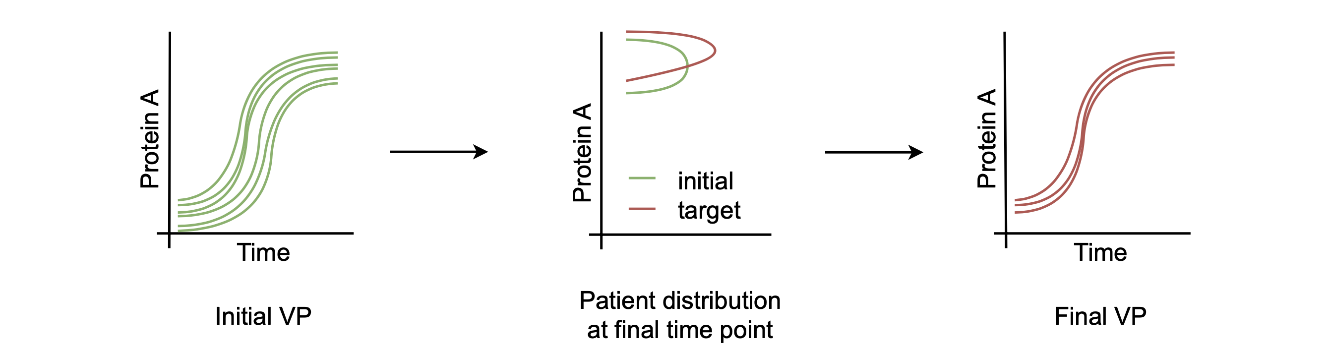
Subsampling
Here we demonstrate the subsampling procedure Discretized Density Sampling (DDS). DDS forms part of the subsampling suite in PumasQSP. For more details on other subsamping strategies see API section).
Julia environment
For this tutorial we will need the following packages:
| Module | Description |
|---|---|
| PumasQSP | PumasQSP is used to formulate the QSP workflow. |
| ModelingToolkit | The symbolic modeling environment |
| DifferentialEquations | The numerical differential equation solvers |
| DataSets | We will load our experimental data from datasets on JuliaHub. |
| CSV | Handling delimited text data |
| DataFrames | Handling tabular data manipulation |
| Plots and StatsPlots | The plotting and visualization libraries used for this tutorial. |
First we prepare the environment by listing the packages we are using within the example.
# Packages used for this example
using PumasQSP
using ModelingToolkit
using DifferentialEquations
using DataSets
using DataFrames
using CSV
using Distributions
using Plots
using StatsPlots
Model and Trials setup
We define our model using ModelingToolkit.jl.
# Model states and their default values
@variables begin
    t
    y1(t) = 1.0
    y2(t) = 0.0
    y3(t) = 0.0
    y4(t) = 0.0
    y5(t) = 0.0
    y6(t) = 0.0
    y7(t) = 0.0
    y8(t) = 0.0057
end

# Model parameters and their default values
@parameters begin
    k1 = 1.71
    k2 = 280.0
    k3 = 8.32
    k4 = 0.69
    k5 = 0.43
    k6 = 1.81
end

# Differential operator
D = Differential(t)

# Differential equations
eqs = [
    D(y1) ~ (-k1*y1 + k5*y2 + k3*y3 + 0.0007),
    D(y2) ~ (k1*y1 - 8.75*y2),
    D(y3) ~ (-10.03*y3 + k5*y4 + 0.035*y5),
    D(y4) ~ (k3*y2 + k1*y3 - 1.12*y4),
    D(y5) ~ (-1.745*y5 + k5*y6 + k5*y7),
    D(y6) ~ (-k2*y6*y8 + k4*y4 + k1*y5 - k5*y6 + k4*y7),
    D(y7) ~ (k2*y6*y8 - k6*y7),
    D(y8) ~ (-k2*y6*y8 + k6*y7)
]

# Model definition
@named model = ODESystem(eqs)
\[ \begin{align} \frac{\mathrm{d} \mathrm{y1}\left( t \right)}{\mathrm{d}t} =& 0.0007 + k5 \mathrm{y2}\left( t \right) + k3 \mathrm{y3}\left( t \right) - k1 \mathrm{y1}\left( t \right) \\ \frac{\mathrm{d} \mathrm{y2}\left( t \right)}{\mathrm{d}t} =& k1 \mathrm{y1}\left( t \right) - 8.75 \mathrm{y2}\left( t \right) \\ \frac{\mathrm{d} \mathrm{y3}\left( t \right)}{\mathrm{d}t} =& - 10.03 \mathrm{y3}\left( t \right) + k5 \mathrm{y4}\left( t \right) + 0.035 \mathrm{y5}\left( t \right) \\ \frac{\mathrm{d} \mathrm{y4}\left( t \right)}{\mathrm{d}t} =& - 1.12 \mathrm{y4}\left( t \right) + k3 \mathrm{y2}\left( t \right) + k1 \mathrm{y3}\left( t \right) \\ \frac{\mathrm{d} \mathrm{y5}\left( t \right)}{\mathrm{d}t} =& - 1.745 \mathrm{y5}\left( t \right) + k5 \mathrm{y6}\left( t \right) + k5 \mathrm{y7}\left( t \right) \\ \frac{\mathrm{d} \mathrm{y6}\left( t \right)}{\mathrm{d}t} =& k1 \mathrm{y5}\left( t \right) + k4 \mathrm{y4}\left( t \right) + k4 \mathrm{y7}\left( t \right) - k5 \mathrm{y6}\left( t \right) - k2 \mathrm{y6}\left( t \right) \mathrm{y8}\left( t \right) \\ \frac{\mathrm{d} \mathrm{y7}\left( t \right)}{\mathrm{d}t} =& - k6 \mathrm{y7}\left( t \right) + k2 \mathrm{y6}\left( t \right) \mathrm{y8}\left( t \right) \\ \frac{\mathrm{d} \mathrm{y8}\left( t \right)}{\mathrm{d}t} =& k6 \mathrm{y7}\left( t \right) - k2 \mathrm{y6}\left( t \right) \mathrm{y8}\left( t \right) \end{align} \]
Subseqeuntly, we create two clinical trial conditions.
# Clinical condition 1
# Load data using DataSets packages
data1 = dataset("pumasqsptutorials/hires_trial_1")

trial1 = SteadyStateTrial(data1, model;
                        params=[k6 => 20.0],
                        alg=DynamicSS(QNDF()),
                        abstol=1e-10,
                        reltol=1e-10
)

# Clinical condition 2
# Load data using DataSets packages
data2 = dataset("pumasqsptutorials/hires_trial_2")

# Create the Trial object for trial 2
trial2 = Trial(data2, model;
                params = [k3 => 4.0, k4 => 0.4, k6 => 8.0],
                tspan = (0.0, 20.0),
                abstol = 1e-10,
                reltol = 1e-10
)
Trial with parameters:
k3 => 4.0
k4 => 0.4
k6 => 8.0.
timespan: (0.0, 20.0)
Using trial1 and trial2, we then define the InverseProblem with a search space.
# Define a search space
example_ss = [k1 => (1.0, 3.0),
              k2 => (200.0, 400.0),
              y1 => (0.0, 3.0)
]

# Create trial collection
trials = SteadyStateTrials(trial1, trial2)

# Create a InverseProblem object
prob = InverseProblem(trials, model, example_ss)
InverseProblem for model with 2 trials optimizing 3 parameters and states.
Lastly, we load a pre-trained Virtual Population object from a file.
# Read Virtual Population from dataset and import as VPResult
data = dataset("pumasqsptutorials/vp")
df = open(IO, data) do io
    CSV.read(io, DataFrame)
end
vp = import_vpop(df, prob)
Virtual population of size 1000.
┌────────────┬───────────┬─────────┐
│ y1(t) │ k1 │ k2 │
├────────────┼───────────┼─────────┤
│ 0.0835802 │ 0.811822 │ 227.6 │
│ 0.00608752 │ 2.27361 │ 238.794 │
│ 0.0265608 │ 1.60797 │ 284.08 │
│ 0.044584 │ 0.357792 │ 262.775 │
│ 0.0310739 │ 0.83363 │ 399.164 │
│ 0.0912289 │ 0.875408 │ 385.448 │
│ 0.147306 │ 0.0344307 │ 317.839 │
│ 0.0881048 │ 0.33897 │ 206.566 │
│ 0.00415461 │ 0.509154 │ 241.224 │
│ 0.0520245 │ 0.342263 │ 242.29 │
│ 0.0394063 │ 1.05342 │ 297.387 │
│ 0.0814158 │ 0.690934 │ 276.569 │
│ 0.0102735 │ 2.35286 │ 271.876 │
│ 0.00790389 │ 2.23132 │ 258.614 │
│ 0.00465267 │ 1.58992 │ 262.58 │
│ 0.0454282 │ 0.149752 │ 325.1 │
│ ⋮ │ ⋮ │ ⋮ │
└────────────┴───────────┴─────────┘
984 rows omitted
Subsampling
The next step is to choose a subsampling algorithm, alg and run the subsampling on vp and our chosen trial. In this case we are considering the second condition, trial2 and the Discretized Density Sampling (DDS) algorithm.
# First set the reference distributions for the considered states
dist1 = TransformedBeta(Beta = Beta(2,6), lb = 0.0, ub = 0.12)
dist4 = TransformedBeta(Beta = Beta(2,5), lb = 0.0, ub = 0.002)
dist5 = TransformedBeta(Beta = Beta(3,3), lb = 0.0, ub = 0.0001)

# Each reference distribution is assigned to a state and describes the desired distribution at timepoint t
ref = [
    y1 => (dist = dist1, t = 20.0),
    y4 => (dist = dist4, t = 20.0),
    y5 => (dist = dist5, t = 20.0)
]

# Set the number of patients to subsample and define the DDS algorithm
subsample_population_size = 400
alg = DDS(reference = ref, n = subsample_population_size, nbins = 20)

# Run subsampling for the second condition
vp_sub = subsample(alg, vp, trial2)
Virtual population of size 400.
┌─────────────┬───────────┬─────────┐
│ y1(t) │ k1 │ k2 │
├─────────────┼───────────┼─────────┤
│ 0.10148 │ 0.284545 │ 385.18 │
│ 0.0454976 │ 0.0448214 │ 309.31 │
│ 0.0870328 │ 0.132543 │ 318.926 │
│ 0.000195905 │ 2.77156 │ 225.468 │
│ 0.0974946 │ 0.177184 │ 318.623 │
│ 0.0844511 │ 0.183531 │ 353.477 │
│ 0.0236881 │ 0.0557557 │ 323.566 │
│ 0.150068 │ 0.203784 │ 364.075 │
│ 0.100219 │ 0.0545585 │ 389.94 │
│ 0.0615442 │ 0.176576 │ 282.144 │
│ 0.0387392 │ 0.0475441 │ 203.244 │
│ 0.0619486 │ 0.0599833 │ 350.541 │
│ 0.107384 │ 0.111168 │ 215.623 │
│ 0.0596616 │ 0.109347 │ 217.981 │
│ 0.141064 │ 0.147734 │ 394.873 │
│ 0.0472182 │ 0.120555 │ 235.432 │
│ ⋮ │ ⋮ │ ⋮ │
└─────────────┴───────────┴─────────┘
384 rows omitted
Visualization
Finally, we can visualize the result of subsampling, by first simulating trial2 using the original vp and the subsampled vp_sub, and then plotting a histogram of the distribution of the considered states y1, y4 and y5.
sim = solve_ensemble(vp, trial2)
df = [DataFrame(sol) for sol in sim]
data = reduce(append!, df)

sim_sub = solve_ensemble(vp_sub, trial2)
df_sub = [DataFrame(sol) for sol in sim_sub]
data_sub = reduce(append!, df_sub)

plt = map(ref) do r
    state = first(r)
    ref_info = last(r)
    timestamp = ref_info.t
    ref_dist = ref_info.dist
    state_data = data[(data.timestamp .== timestamp), string(state)]
    state_data_sub = data_sub[(data_sub.timestamp .== timestamp), string(state)]
    histogram(state_data, normalize = true, nbins = 50, alpha = 0.3, label = "Plausible Population (PP)", title = string(state))
    histogram!(state_data_sub, normalize = true, nbins = 50, alpha = 0.3, label = "Subsampled PP - Virtual Population")
    histogram!(rand(ref_dist, 1_000), normalize = true, nbins = 50, alpha = 0.3, label = "Reference")
end
plot(plt..., layout = (3, 1), legendfontsize = 7)
As we can see from the plot, the subsampled Virtual Population is closer to the reference distribution for all three states than the original Plausible Population.