Virtual Population
In PumasQSP, virtual populations are generated using the vpop function on an InverseProblem. The result of a vpop is a set of parameters which sufficiently fit all trials to their respective data simultaniously. Note that in the QSP field, this initial poulation is sometimes referred to as a plausible patient population, which can be subsequently subsampled to a virtual population following the subsampling API.
The vpop Function
JuliaSimModelOptimizer.vpop — Functionvpop(prob, alg; population_size)Create a plausible population of the given size using the method specified by alg.
Arguments
prob: anInverseProblemobjectalg: a parametric uncertainty quantification algorithm, e.g.StochGlobalOptorMCMCOpts
Keyword Arguments
population_size: Required. Number of plausible patients to generate.adtype: Automatic differentiation choice, see the Optimization.jl docs
for details. Defaults to AutoForwardDiff().
Stochastic Optimization
If alg is a StochGlobalOpt method, the optimization algorithm runs until convergence or until maxiters has been reached. This process is repeated a number of times equal to population_size to create a plausible population.
Markov Chain Monte Carlo (MCMC)
If alg is an MCMCOpt method, the plausible population is produced by drawing samples equal to population_size from the posterior samples that the method has computed. This way, the variability in the plausible population depends on the uncertainty (variance) of the posterior distribution.
Note: It is recommended that maxiters > population_size for MCMCOpt methods, so that the same parameter values are not sampled multiple times in the vpop. Drawing a larger number of maxiters samples also helps to better characterize the variability around each parameter.
Optimization Methods
The following are the choices of AbstractVpopAlgorithm which are available for controlling the virtual population generation process:
JuliaSimModelOptimizer.StochGlobalOpt — TypeStochGlobalOpt(; method = SingleShooting(optimizer = BBO_adaptive_de_rand_1_bin_radiuslimited(),
maxiters = 10_000),
parallel_type=EnsembleSerial())A stochastic global optimization method.
Keyword Arguments
parallel_type: Choice of parallelism. Defaults toEnsembleSerial()or serial computation. For more information on ensemble parallelism types, see the ensemble types from SciMLmethod: a calibration algorithm to use during the runs. Defaults toSingleShooting(optimizer=BBO_adaptive_de_rand_1_bin_radiuslimited(), maxiters=10_000). i.e. single shooting method with a black-box differential evolution method from BlackBoxOptimization. For more information on choosing optimizers, see Optimization.jl.
JuliaSimModelOptimizer.MCMCOpt — TypeMCMCOpt(; maxiters, discard_initial = max(Int(round(maxiters/2)), 1000),
parallel_type = EnsembleSerial(), sampler = Turing.NUTS(0.65),
hierarchical = false)A Markov-Chain Monte Carlo (MCMC) method for solving the inverse problem. The method approximates the posterior distribution of the model parameters given the data with a number of samples equal to maxiters.
Keyword Arguments
maxiters: Required. Represents the number of posterior distribution samples.parallel_type: Choice of parallelism. Defaults toEnsembleSerial()or serial computation. Determines the number of chains of samples that will be drawn. For more information on ensemble parallelism types, see the ensemble types from SciML.discard_initial: The number of initial samples to discard. Defaults to the maximum between half of themaxiterssamples and 1000, as a general recommendation. This default is the same as the number of samples thatsamplerdraws during its warm-up phase, when the defaultNUTSsampler is used.sampler: The sampler used for the MCMC iterations. Defaults toTuring.NUTSfor the No-U-Turn Sampler variant of Hamiltonian Monte Carlo. For more information on sampler algorithms, see the Turing.jl documentationhierarchical: Defaults tofalse. Controls whether hierarchical MCMC inference will be used. If it is set totrue, eachTrialobject of theInverseProblemis treated as a separate subject and all subjects are assumed to come from the same population distribution. Population-level parameters are generated internally and their posterior is also inferred from data. If it is set tofalse, it is assumed that the same parameters are used for each subject and thus inference is performed on a lower-dimensional space.
Result Types
PumasQSP.VpopResult — TypeVpopResultThe structure contains the result of a plausible population when a StochGlobalOpt method was used to generate the population. To export results to a DataFrame use DataFrame(vp) and to plot them use plot(vp, trial), where vp is the VpopResult and trial is the AbstractExperiment, whose default parameter (or initial condition) values will be used.
JuliaSimModelOptimizer.MCMCResult — TypeMCMCResultThe structure contains the result of a plausible population when an MCMCOpt method was used to generate the population. To export results to a DataFrame use DataFrame(vp) and to plot them use plot(vp, trial), where vp is the VpopResult and trial is the AbstractExperiment, whose default parameter (or initial condition) values will be used.
The original Markov chain object that the MCMC method generated can be accessed using vp.original. This object contains summary statistics for each parameter and diagnostics of the MCMC method (e.g. Rhat and Effective Sample Size). See the MCMCChains.jl documentation for more information about diagnostic checks that can be run on vp.original.
Importing Virtual Populations
If a virtual popualtion was generated in some alternative way, PumasQSP still allows for importing these values into a VpopResult to enable using the virtual population analysis workflow. This is done via the following function:
PumasQSP.import_vpop — Functionimport_vpop(vp, prob)Import a Plausible Population object (VpopResult) from tabular data.
Arguments
vp: tabular data that contains the parameters of the population. This could be e.g aDataFrameor aCSV.File.prob: anInverseProblemobject.
Analyzing Virtual Population Results
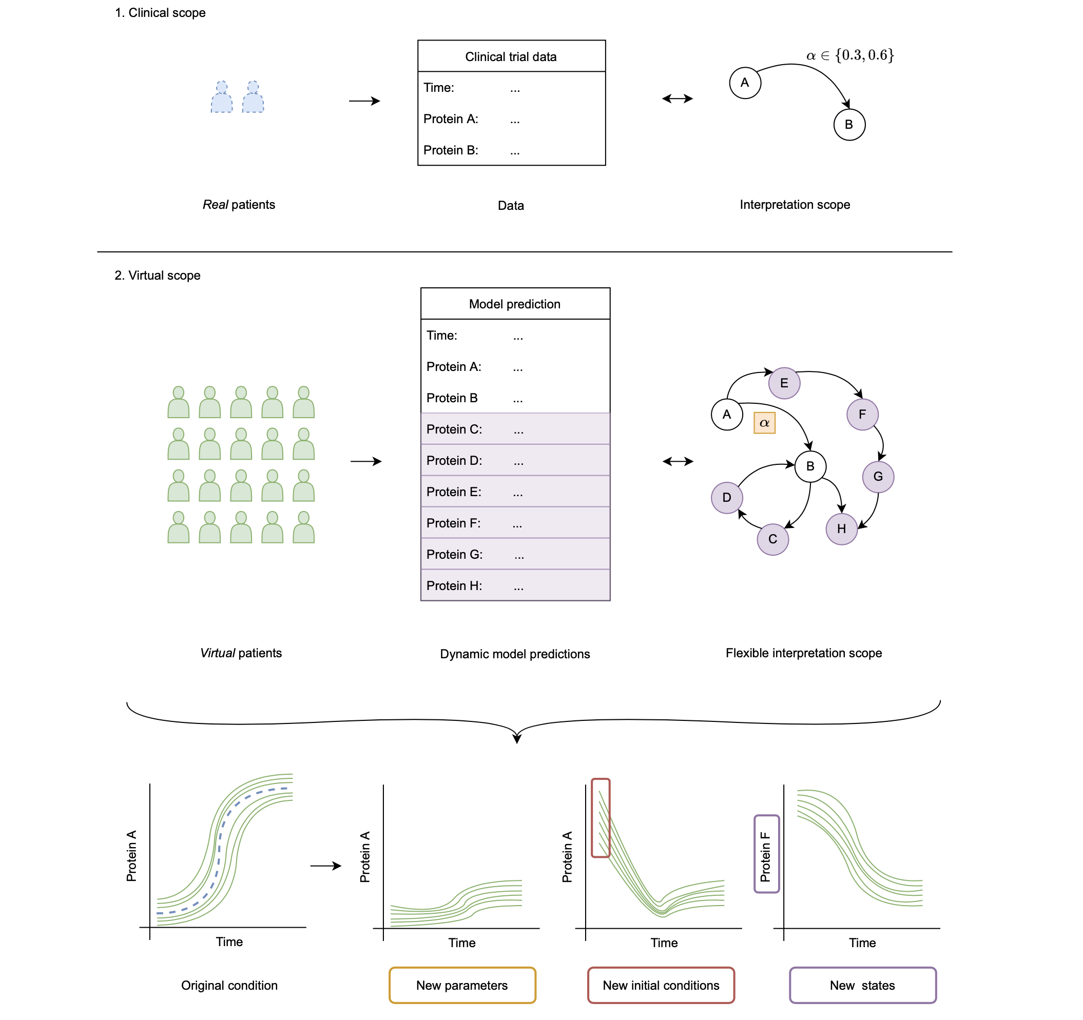
Once a virtual population is generated given some clinical data, we can use it to expand our analysis scope to dimensions where, for example, experimental data collection is difficult. This objective is schematically shown in the figure below. Here, we summarise three groups:
- We can use the VP to model the system for new values of model parameters. Note that here we refer to model parameters not as parameters that specify a patient, but other, independent parameters of the model. As an example we have the reaction rate α.
- We can use the VP to model the system for new initial conditions for the observed states of the sytem. Here, this relates to Protein A and B.
- We can use the VP to model states of the system that have not been observed. These are Protein C to H in this example.
The following functions enable such analyses:
JuliaSimModelOptimizer.solve_ensemble — Functionsolve_ensemble(vp, trial)Create and solve an EnsembleProblem descrbing the patients in the plausible population vp and using trial for the parameter and initial condition values.