Identifiability Analysis of in-vitro Pitavastatin Hepatoc Uptake
In this tutorial we demonstrate how to use Pumas-QSP's tooling to identify structural and practical identifiability using a virtual populations analysis mixed with symbolic tooling.
Motivation
Identifiability is a requirement for many algorithms used in pharmacometrics, such as those used in nonlinear mixed effects modeling (NLME). Whenever the identifiability criteria are not met, QSP workflows based on different methodology (e.g. global optimization procedures), are necessary in order to avoid a systematic underestimation of uncertainty.
Julia environment
For this tutorial we will need the following packages:
| Module | Description |
|---|---|
| PumasQSP | PumasQSP is used to formulate our problem and perform automated model discovery |
| ModelingToolkit | The symbolic modeling environment |
| DifferentialEquations | The numerical differential equation solvers |
| DataSets | We will load our experimental data from datasets on JuliaHub |
| DataFrames | Handling tabular data manipulation |
| StableRNGs | Stable random seeding |
| StatsPlots | The plotting and visualization library |
First we prepare the environment by listing the packages we are using within the example.
#Packages used for this example
using PumasQSP
using ModelingToolkit
using DifferentialEquations
using DataSets
using DataFrames
using StructuralIdentifiability: assess_identifiability, assess_local_identifiability
using StatsPlots
using Random
Model setup
As a demonstration, we will use a pharmacokinetic model of in-vitro Pitavastatin hepatoc uptake [1]. This is a system of equations, as shown below, contains two states, one observable and six unknown parameters as shown below.
\[\begin{aligned} \frac{dx_1}{dt} &= k_3 x_3 - r_3 x_1 - k_1 x_1 (T_\theta - d + x_1 + x_3) + r_1 (d - x_1 - x_3) \\ \frac{dx_3}{dt} &= r_3 x_1 - k_3 x_3 + k_2 (d - x_1 - x_3) \\ y &= k (d - x_1) \end{aligned}\]
The system of ODEs is a mass-action model where $T_\theta$ is the total number of transporter binding sites, and other parameters like ${k_1, r_1, k_2, k_3, r_3}$, are the reaction constants. The $d$ is the initial concentration value of the medium where the hepatocytes initially reside before the trial, which is known prior to conducting the trial. The unknown concentrations in each of the compartments inside the hepatocyte cell, x1 and x3, is modeled by the underlying differential equations. The k is the observation gain constant, which is used to measure the observed variable y.
# States of the model
k = 1
d = 5
@variables begin
	t
	x1(t) = k*d
	x3(t) = 0
	y(t)
end

# Parameters of the model
@parameters begin
	k₁ = 0.5
	k₂ = 0.5
	k₃ = 0.8
	r₁ = 0.8
	r₃ = 1.2
	T₀ = 3.5
end

# Equations of the model
D = Differential(t)
eqs = [
	    D(x1) ~ (k₃ * x3 - r₃ * x1 - k₁ * x1 * (T₀ - d + x1 + x3) + r₁ * (d - x1 - x3)),
	    D(x3) ~ (r₃ * x1 - k₃ * x3 + k₂ * (d - x1 - x3)),
	]
obs_eq = [y ~ k * (d - x1)]
measured_quantities = [y ~ k * (d - x1)]

# Model
@named model = ODESystem(eqs; observed = obs_eq)
\[ \begin{align} \frac{\mathrm{d} \mathrm{x1}\left( t \right)}{\mathrm{d}t} =& r_1 \left( 5 - \mathrm{x1}\left( t \right) - \mathrm{x3}\left( t \right) \right) + k_3 \mathrm{x3}\left( t \right) - r_3 \mathrm{x1}\left( t \right) - k_1 \left( -5 + T_0 + \mathrm{x1}\left( t \right) + \mathrm{x3}\left( t \right) \right) \mathrm{x1}\left( t \right) \\ \frac{\mathrm{d} \mathrm{x3}\left( t \right)}{\mathrm{d}t} =& k_2 \left( 5 - \mathrm{x1}\left( t \right) - \mathrm{x3}\left( t \right) \right) + r_3 \mathrm{x1}\left( t \right) - k_3 \mathrm{x3}\left( t \right) \end{align} \]
Assessing Structural Identifiability
We will start our analysis with by using structural identifiability analysis tooling. Structural identifiability analysis is symbolic and assumes perfect measurement. It calculates whether it's even mathematically possible to identify given parameters with the chosen observables even when there is infinite data on the observables. While a good starting point for understanding parametric identifiability, this method is unable to say whether the true amount of data is sufficient for practically identifying the parameters from data (i.e. it does not do practical identifiability analysis). Also, such a symbolic method is difficult to scale to high dimensions, and thus is only possible on small models such as one demonstrated here.
To perform structural identifiability analysis, we will use assess_local_identifiability from StructuralIdentifiability.jl as follows.
# Local Identifiability Check
assess_local_identifiability(model, measured_quantities = measured_quantities,p = 0.99)
Dict{SymbolicUtils.BasicSymbolic{Real}, Bool} with 8 entries:
r₃ => 1
T₀ => 1
r₁ => 1
k₃ => 1
k₂ => 1
k₁ => 1
x1(t) => 1
x3(t) => 1From above observations we can see that all the parameters are found to be locally identifiabile, and this is validated from the uniquely identifiable peaks for each of the parameters, that is described by histogram plots below. We can also run a global identifiable check as defined below, where it will first run the local identifiable checks, and then compute the Wronskians, to proceed for the global identifiability checks, which adds overheads to the overall compute time. Depending on the tolerance for the probability of accuracy with which the parameters can be identifiable, can also effect the compute-time taken to complete the identifiability check, for example changing the probability kwarg to p=0.9, can significantly reduce the run-time.
# Global Identifiability Check
assess_identifiability(model, measured_quantities = measured_quantities,p = 0.99)
Dict{SymbolicUtils.BasicSymbolic{Real}, Symbol} with 6 entries:
r₃ => :globally
T₀ => :globally
r₁ => :globally
k₃ => :globally
k₂ => :globally
k₁ => :globallyAnalyzing Practical Identifiability via Virtual Populations
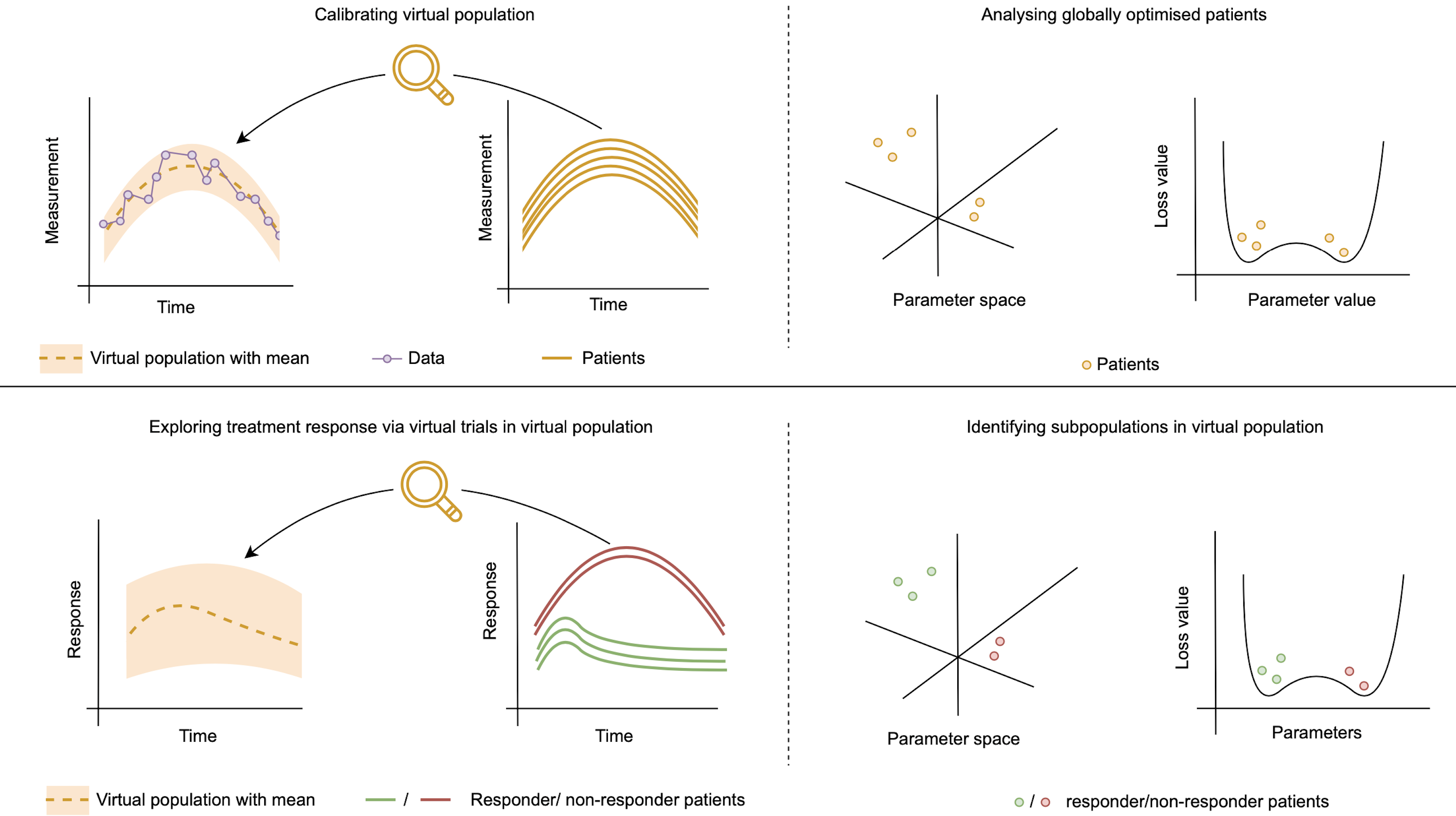
Knowing that the model is structurally identifiable means that with noise-less infinite data on the chosen observables, the parameter values are expected to be exactly identifiable. However, in practice our data has noise and is not infinite. Thus we wish to understand how identifiable our parameters really are given the data we have on hand. This is one way to define practical identifiability analysis. While there are many ways to perform a practical identifiability analysis, one simple way is to use virtual populations to find an ensemble of fitting parameters and analyzing the resulting distribution of parameters which all equally fit the data. We will demonstrate this using Pumas-QSP's vpops functionality.
First we prepare the arguments describing the model configuration presented in the trial of interest and load the respective dataset.
# Trial configuration
inits = [x1 => k * d]
ps = [k₁ => 0.6,
	    k₂ => 0.7,
	    k₃ => 0.9,
	    r₁ => 1,
	    r₃ => 1.4,
	    T₀ => 4]
tspan = (0.0, 1.0)

# Load dataset
data = dataset("pumasqsptutorials/Pitavastatin_hepatoc_uptake_data")
name = "pumasqsptutorials/Pitavastatin_hepatoc_uptake_data"
uuid = "b29f02e4-e94a-44d0-947b-269b02db6e23"
description = "For example \"Identifiability Analysis of in-vitro Pitavastatin Hepatoc Uptake\" in PumasQSP."
type = "Blob"
[storage]
driver = "JuliaHubDataRepo"
bucket_region = "us-east-1"
bucket = "internaljuilahubdatasets"
credentials_url = "https://internal.juliahub.com/datasets/b29f02e4-e94a-44d0-947b-269b02db6e23/credentials"
prefix = "datasets"
vendor = "aws"
type = "Blob"
[storage.juliahub_credentials]
auth_toml_path = "/home/github_actions/actions-runner-1/home/.julia/servers/internal.juliahub.com/auth.toml"
[[storage.versions]]
blobstore_path = "u1"
date = "2023-08-24T22:41:31.332+00:00"
size = 1102
version = 1
Subesquently, we define the Trial.
trial = Trial(data, model;
        u0 = inits,
        params = ps ,
		save_names = [y],
        tspan = tspan)
Trial with parameters:
k₁ => 0.6
k₂ => 0.7
k₃ => 0.9
r₁ => 1.0
r₃ => 1.4
T₀ => 4.0 and initial conditions:
x1(t) => 5.
timespan: (0.0, 1.0)
Creating the InverseProblem
After we have built the Trial, the next step is to define the InverseProblem, i.e. specifying the parameters we want to optimize and the search space in which we want to look for them.
Random.seed!(1234)
prob = InverseProblem(trial, model, [
			        k₁ => (0.5,1),
			        k₂ => (0.5,1),
			        k₃ => (0.5,1),
			        r₁ => (0.8,1.2),
			        r₃ => (1.2,1.6),
	  	            T₀ => (3.5,4.5)
			])

vp = vpop(prob, StochGlobalOpt(maxiters = 2_000), population_size=4000)
Virtual population of size 4000 computed in 15 minutes and 46 seconds.
┌──────────┬──────────┬──────────┬──────────┬─────────┬─────────┐
│ k₁ │ k₂ │ k₃ │ r₁ │ r₃ │ T₀ │
├──────────┼──────────┼──────────┼──────────┼─────────┼─────────┤
│ 0.888552 │ 0.790247 │ 0.611315 │ 1.02436 │ 1.52653 │ 3.84786 │
│ 0.824606 │ 0.560189 │ 0.812509 │ 0.933624 │ 1.30911 │ 3.7266 │
│ 0.840809 │ 0.77776 │ 0.778959 │ 1.05985 │ 1.42813 │ 3.74966 │
│ 0.93697 │ 0.812642 │ 0.685942 │ 1.07831 │ 1.40037 │ 3.80405 │
│ 0.613054 │ 0.702493 │ 0.524314 │ 0.89945 │ 1.3815 │ 3.84694 │
│ 0.629345 │ 0.593326 │ 0.70111 │ 0.889245 │ 1.5454 │ 4.37761 │
│ 0.575516 │ 0.506559 │ 0.871397 │ 0.85805 │ 1.45099 │ 3.76198 │
│ 0.759263 │ 0.688281 │ 0.642758 │ 1.15899 │ 1.21588 │ 3.61573 │
│ 0.679271 │ 0.662836 │ 0.933642 │ 0.905037 │ 1.34672 │ 3.65136 │
│ 0.983124 │ 0.88132 │ 0.971363 │ 0.962859 │ 1.42613 │ 3.67558 │
│ 0.66819 │ 0.633773 │ 0.710946 │ 1.01634 │ 1.28812 │ 3.83419 │
│ 0.760087 │ 0.665976 │ 0.630409 │ 0.943526 │ 1.53615 │ 4.31732 │
│ 0.624169 │ 0.684434 │ 0.825686 │ 1.03035 │ 1.59459 │ 4.47193 │
│ 0.970854 │ 0.840648 │ 0.819677 │ 1.00797 │ 1.55905 │ 4.16707 │
│ 0.641727 │ 0.761431 │ 0.844342 │ 0.987719 │ 1.38037 │ 3.52153 │
│ 0.781472 │ 0.529396 │ 0.647244 │ 0.844894 │ 1.41966 │ 4.45383 │
│ ⋮ │ ⋮ │ ⋮ │ ⋮ │ ⋮ │ ⋮ │
└──────────┴──────────┴──────────┴──────────┴─────────┴─────────┘
3984 rows omitted
The InverseProblem consists of a collection of trials which define a multi-simulation optimization problem. The solution to an inverse problem are the "good parameters" which make the simulations simultaneously fit their respective data sufficiently well. In this context, we have only created a single trial.
Validating the identifiability observations from StructuralIdentifiablity.jl
We visualize results via density plots.
plot(vp, layout=(2,3), show_comparision_value = [0.6, 0.7, 0.9, 1, 1.4, 4], max_freq = [500, 500, 500, 500, 500, 500], legend = :outerright, size = (3000, 1000))
From the generated histogram plot observations, we can justify that each of the parameters have peaks that can be uniquely identifiable. Hence, we can understand that it represents a practically identifiable system. We can notice a few local peaks, which may occur due to practical identifiability as we lack sufficient data. Let us look at the data fit using the generated vpop members below.
Visualizing the accuracy in data fit out of the vpop members
confidenceplot(trial, vp, confidence = 0,legend = true)
As we can clearly see that the degree of cost in the data-fit looks sufficiently reasonable for the worst level of confidence that refers to the worst case parameters that we can have among all the virtual population members. We can thus conclude that our model can identify the parameters very well.
- 1Thomas R. B. Grandjean et al., "Structural Identifiability and Indistinguishability Analyses of in vitro Pitavastatin Hepatic Uptake", IFAC Proceedings Volumes, 2012.