Virtual Population: Hierarchical MCMC
The problem of virtual population generation has a natural hierarchical structure. As depicted in the following figure, virtual patients belong to a virtual population. In a probabilistic sense, we can say that the parameters of virtual patients are samples, generated from population distributions.
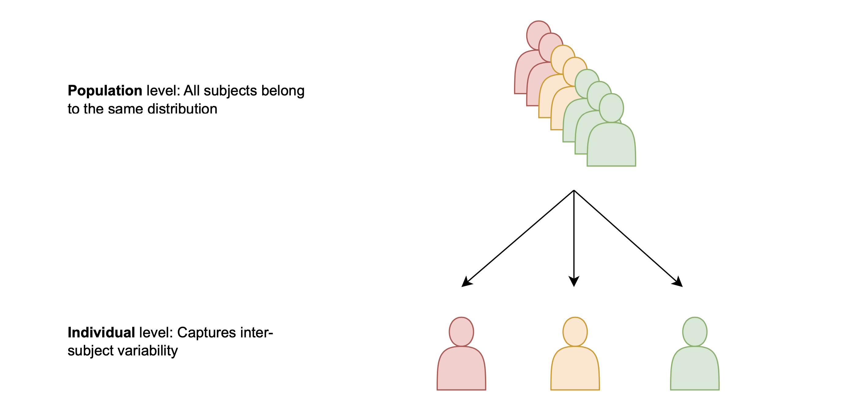
Hierarchical MCMC methods are a family of approximate Bayesian inference methods that explicitly contain a hierarchical structure, like the one in the figure. When using Hierarchical MCMC inference in Pumas-QSP, population-level parameters are inferred at the same time as patient-level parameters and other noise parameters. The population-level parameters are the ones that define the population distributions, out of which virtual patients are sampled. By approximating the posterior distribution of population-level parameters accurately, Pumas-QSP can generate any arbitrary number of virtual patients in the same amount of time.
The following tutorial contains all steps for generating a virtual population by hierarchical MCMC inference.
Julia environment
For this tutorial we will need the following packages:
| Module | Description |
|---|---|
| PumasQSP | PumasQSP is used to formulate the QSP workflow. |
| ModelingToolkit | The symbolic modeling environment |
| DifferentialEquations | The numerical differential equation solvers |
| DataSets | We will load our experimental data from datasets on JuliaHub. |
| DataFrames | Handling tabular data manipulation |
| Turing | Bayesian inference with probabilistic programming |
| Plots and StatsPlots | The plotting and visualization libraries used for this tutorial. |
First we prepare the environment by listing the packages we are using within the example.
# Packages used for this example
using PumasQSP
using ModelingToolkit
using DifferentialEquations
using DataSets
using DataFrames
using CSV
using Turing
using Plots
using StatsPlots
Model setup
As the example model we are using the Hires model with eight variables. Their dynamics are described by eight equations and default values are set for the variables and parameters. We use the ModelingTookit.jl package to specify the model in Julia.
# Model states and their default values
@variables begin
    t
    y1(t) = 1.0
    y2(t) = 0.0
    y3(t) = 0.0
    y4(t) = 0.0
    y5(t) = 0.0
    y6(t) = 0.0
    y7(t) = 0.0
    y8(t) = 0.0057
end

# Model parameters and their default values
@parameters begin
    k1 = 1.71
    k2 = 280.0
    k3 = 8.32
    k4 = 0.69
    k5 = 0.43
    k6 = 1.81
end

# Differential operator
D = Differential(t)

# Differential equations
eqs = [
    D(y1) ~ (-k1*y1 + k5*y2 + k3*y3 + 0.0007),
    D(y2) ~ (k1*y1 - 8.75*y2),
    D(y3) ~ (-10.03*y3 + k5*y4 + 0.035*y5),
    D(y4) ~ (k3*y2 + k1*y3 - 1.12*y4),
    D(y5) ~ (-1.745*y5 + k5*y6 + k5*y7),
    D(y6) ~ (-k2*y6*y8 + k4*y4 + k1*y5 - k5*y6 + k4*y7),
    D(y7) ~ (k2*y6*y8 - k6*y7),
    D(y8) ~ (-k2*y6*y8 + k6*y7)
]

# Model definition
@named model = ODESystem(eqs)
\[ \begin{align} \frac{\mathrm{d} \mathrm{y1}\left( t \right)}{\mathrm{d}t} =& 0.0007 + k5 \mathrm{y2}\left( t \right) + k3 \mathrm{y3}\left( t \right) - k1 \mathrm{y1}\left( t \right) \\ \frac{\mathrm{d} \mathrm{y2}\left( t \right)}{\mathrm{d}t} =& k1 \mathrm{y1}\left( t \right) - 8.75 \mathrm{y2}\left( t \right) \\ \frac{\mathrm{d} \mathrm{y3}\left( t \right)}{\mathrm{d}t} =& - 10.03 \mathrm{y3}\left( t \right) + k5 \mathrm{y4}\left( t \right) + 0.035 \mathrm{y5}\left( t \right) \\ \frac{\mathrm{d} \mathrm{y4}\left( t \right)}{\mathrm{d}t} =& - 1.12 \mathrm{y4}\left( t \right) + k3 \mathrm{y2}\left( t \right) + k1 \mathrm{y3}\left( t \right) \\ \frac{\mathrm{d} \mathrm{y5}\left( t \right)}{\mathrm{d}t} =& - 1.745 \mathrm{y5}\left( t \right) + k5 \mathrm{y6}\left( t \right) + k5 \mathrm{y7}\left( t \right) \\ \frac{\mathrm{d} \mathrm{y6}\left( t \right)}{\mathrm{d}t} =& k1 \mathrm{y5}\left( t \right) + k4 \mathrm{y4}\left( t \right) + k4 \mathrm{y7}\left( t \right) - k5 \mathrm{y6}\left( t \right) - k2 \mathrm{y6}\left( t \right) \mathrm{y8}\left( t \right) \\ \frac{\mathrm{d} \mathrm{y7}\left( t \right)}{\mathrm{d}t} =& - k6 \mathrm{y7}\left( t \right) + k2 \mathrm{y6}\left( t \right) \mathrm{y8}\left( t \right) \\ \frac{\mathrm{d} \mathrm{y8}\left( t \right)}{\mathrm{d}t} =& k6 \mathrm{y7}\left( t \right) - k2 \mathrm{y6}\left( t \right) \mathrm{y8}\left( t \right) \end{align} \]
We are considering five patients within the same clinical condition. We first load timeseries data from datasets and then create Trial objects to describe each patient.
N_subjects = 5

# Model solve options
alg = Rodas4P()
reltol = 1e-9
abstol = 1e-9

# Initialize Vector of Trials
trials = []
# Iterate over patients to create and collect Trial objects
for i = 1 : N_subjects
    # Read data from a patient
    patient_dataset = dataset("pumasqsptutorials/patient_$i")
    data = open(IO, patient_dataset) do io
        CSV.read(io, DataFrame)
    end
    # Extract timespan from "timestamp" column in data
    tspan = (first(data[!,:timestamp]), last(data[!,:timestamp]))

    # Define a Trial object for a patient
    trial = Trial(
        data,
        model;
        tspan,
        noise_priors = Exponential(0.1),
        alg,
        reltol,
        abstol
    )

    # Collect a patient's Trial object in a Vector
    push!(trials, trial)
end
Analysis
Next we define the InverseProblem. For this we need a search space, which holds lower and upper boundaries for all parameters and/or initial conditions to be inferred.
In hierarchical MCMC each parameter and/or initial condition to be inferred is assigned a prior distribution and this distribution is bounded by the respective search space bounds. These prior distributions are adaptive because the parameters that define their shape are themselves part of the inference problem instead of numbers, known as population-level parameters or hyperparameters.
So overall, in hierarchical Bayesian inference, we are approximating a posterior distribution over the QSP model parameters, the noise parameters for each patient, and the population-level parameters that define the shape of the distribution of QSP model parameters.
Pumas-QSP builds the hierarchical structure mentioned in the introduction internally, by introducing two population-level parameters for each parameter in the search space. These two parameters are the $\alpha$ and $\beta$ of a TransformedBeta distribution, which is assumed to be the population distribution of the respective parameter in the search space.
search_space = [
    y1 => (0.0, 1.3),
    k1 => (0.0, 1.9),
    k2 => (200.0, 250.0)
]

prob = InverseProblem(trials, model, search_space)
InverseProblem for model with 5 trials optimizing 3 parameters and states.
In this example, we want to infer the initial condition of y1 and the parameters k1 and k2 of the Hires model. Pumas-QSP will then generate six population-level parameters and then use these to parameterize TransformedBeta distributions and sample virtual patient parameters out of them.
Once the QSP model and all trials are defined, the package can generate potential patients, i.e. find parameter combinations for the provided model, which describe the trial data sufficiently well. Particularly in the case of hierarchical MCMC methods, the posterior distribution of the population-level parameters given the data will be approximated in a sampling-based manner.
# Set the hierarchical keyword argument to true for hierarchical inference
alg = MCMCOpt(maxiters=100, hierarchical = true)

# Generate potential population
vp = vpop(prob, alg; population_size = 200)
MCMC result of length 200 computed in 20 minutes and 29 seconds.
┌──────────┬──────────┬─────────┐
│ y1(t) │ k1 │ k2 │
├──────────┼──────────┼─────────┤
│ 0.972144 │ 0.627571 │ 218.415 │
│ 1.12543 │ 0.916419 │ 238.193 │
│ 1.17381 │ 1.26965 │ 246.615 │
│ 1.24131 │ 0.843485 │ 233.744 │
│ 1.29245 │ 1.12381 │ 233.469 │
│ 1.25288 │ 1.40784 │ 249.984 │
│ 0.586931 │ 0.747222 │ 245.185 │
│ 1.2576 │ 1.2655 │ 225.464 │
│ 1.29488 │ 0.999786 │ 248.236 │
│ 1.2735 │ 1.56339 │ 223.471 │
│ 1.21868 │ 1.20947 │ 248.168 │
│ 1.29365 │ 1.26381 │ 232.892 │
│ 1.29872 │ 1.0904 │ 245.785 │
│ 1.27383 │ 0.760978 │ 247.287 │
│ 1.18415 │ 1.42469 │ 221.134 │
│ 1.29928 │ 0.899552 │ 232.14 │
│ ⋮ │ ⋮ │ ⋮ │
└──────────┴──────────┴─────────┘
184 rows omitted
Finally, the original MCMCChain object that was created during Bayesian inference can be accessed via
vp.originalChains MCMC chain (100×23×1 Array{Float64, 3}):
Iterations = 1:1:100
Number of chains = 1
Samples per chain = 100
Wall duration = 1216.07 seconds
Compute duration = 1216.07 seconds
parameters = α_y1(t), α_k1, α_k2, β_y1(t), β_k1, β_k2, noise[1], noise[2], noise[3], noise[4], noise[5]
internals = lp, n_steps, is_accept, acceptance_rate, log_density, hamiltonian_energy, hamiltonian_energy_error, max_hamiltonian_energy_error, tree_depth, numerical_error, step_size, nom_step_size
Summary Statistics
parameters mean std mcse ess_bulk ess_tail rhat e ⋯
Symbol Float64 Float64 Float64 Float64 Float64 Float64 ⋯
α_y1(t) 5.5400 0.0253 0.0223 1.4113 9.7038 2.1569 ⋯
α_k1 5.9479 0.0113 0.0040 8.3632 17.3961 1.4127 ⋯
α_k2 2.2139 0.0024 0.0016 2.6224 21.0246 1.4186 ⋯
β_y1(t) 0.5703 0.0012 0.0006 5.9493 21.5920 1.1375 ⋯
β_k1 4.0456 0.0136 0.0078 4.2546 10.6111 1.3929 ⋯
β_k2 0.7355 0.0010 0.0006 3.3409 15.1573 1.2687 ⋯
noise[1] 0.0000 0.0000 0.0000 1.4032 NaN 2.1668 ⋯
noise[2] 0.0000 0.0000 0.0000 1.5138 12.2836 1.9232 ⋯
noise[3] 0.0000 0.0000 0.0000 1.8876 17.3961 1.5680 ⋯
noise[4] 0.0001 0.0000 0.0000 1.5248 6.6729 1.9295 ⋯
noise[5] 0.0000 0.0000 0.0000 1.4832 12.2836 1.9609 ⋯
1 column omitted
Quantiles
parameters 2.5% 25.0% 50.0% 75.0% 97.5%
Symbol Float64 Float64 Float64 Float64 Float64
α_y1(t) 5.5113 5.5176 5.5353 5.5674 5.5831
α_k1 5.9251 5.9396 5.9486 5.9577 5.9642
α_k2 2.2087 2.2121 2.2145 2.2153 2.2189
β_y1(t) 0.5687 0.5695 0.5699 0.5712 0.5726
β_k1 4.0280 4.0345 4.0430 4.0615 4.0681
β_k2 0.7334 0.7351 0.7355 0.7361 0.7374
noise[1] 0.0000 0.0000 0.0000 0.0000 0.0000
noise[2] 0.0000 0.0000 0.0000 0.0000 0.0000
noise[3] 0.0000 0.0000 0.0000 0.0000 0.0000
noise[4] 0.0001 0.0001 0.0001 0.0001 0.0001
noise[5] 0.0000 0.0000 0.0000 0.0000 0.0000
This MCMCChain object does not contain the patient-level parameters, as these are not used to generate virtual patients. The population-level parameters, $\alpha$ and $\beta$, for each model parameter (k1 and k2) and initial condition (y1) are included as these will be used to sample virtual patients.
Additionally, the noise parameters are shown as an estimate of the measurement noise for each patient. It was assumed that the same noise parameter is applied to all states, so there is only one index for patient in noise. See the MCMC tutorial for a more elaborate choice of noise parameters that could be applied here too.
Visualization
We can conveniently analyze and visualize the results by relying on the ploting recipes of Pumas-QSP.
# Viusalization (1/2): Simulation results for Patient 2
plot(vp, trials[2], legend = :outerright, grid = "off")
# Viusalization (2/2): Parameters
params = DataFrame(vp)[!,"y1(t)"]
plt = violin(params, grid = :off, legend = :outerright, label = "VP", ylabel = "y1", color = "purple")
Simulating Virtual Trials
Once we have created and validated our VP, we can use it to explore the system for new clinical conditions. For instance, what would happen to patient 2 if the initial condition for y3 and the parameter k1 were different? For this, we can use the virtual_trial function.
# Create virtual trial
vt = virtual_trial(trials[2], model;
	                u0 = [y3 =>2.1],
	                params = [k1 => 1.9],
	                tspan = (0, 100))

# Visualize simulation results
plot(vp, vt, legend = :outerright, grid = "off")