PEtab Format
Motivation
With the PEtab format([1]) users can specify probabilistically motivated (log-likelihood and log-posterior) objective functions for parameter estimation problems in systems biology. PEtab offers a zero-code way to define an InverseProblem in PumasQSP.
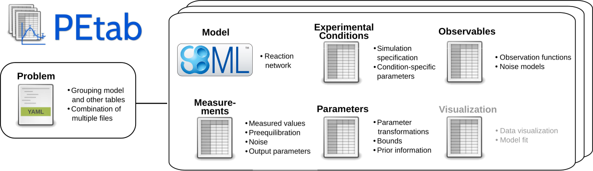
One of the big advantages of the PEtab format is its modular design that facilitates reusing and modifying the inverse problem. In particular PEtab defines
- an (SBML) model that describes the system dynamics.
- a so-called observation model that describes how system states map to experimental readouts.
- a so-called noise model to define the likelihood of the data given the expected (i.e. simulated) observation.
- a treatment model, that defines perturbations of the model.
Here, we will first provide a high-level explanation of the PEtab format, followed by a tutorial for creating an inverse problem.
Background: The PEtab format
The two most critical parts to define an inverse problem are the model and experimental data. In PEtab, the model is specified in the Systems Biology Markup Language (SBML). The experimental data is defined in a measurement table. In its simplest form and interpreted via DataFrames.jl, it looks like this:
| Row | observableId | simulationConditionId | measurement | time |
|---|---|---|---|---|
| String | String | Any | Any | |
| 1 | obs_A | trial1 | 3.5 | 0.0 |
| 2 | ... | ... | ... | ... |
You will first notice, that the measurement table is in the stacked or long form. You may also wonder what the entries in the observableId, and conditionId mean. These entries have to be defined in an observable table and a condition table. In this sense, a PEtab problem is like a Relational Database.
Following this concept, PEtab also specifies the search space and other parameter-related information in a separate parameter table. A detailed description of all the tables, columns and their relations can be found in the documentation of the PEtab data format. If this all sounds abstract, the following tutorial will make the format and its application to QSP more concrete.
 Note that PumasQSP does currently not support Preequilibration, time point-specific observable and noise parameter overrides as well as the visualization table.
PumasQSP extends the core PEtab features with
- A dosing table.
- Use of ModelingToolkit
ODESystems instead of SBML models. - Support of
observableIds in thenoiseFormula.
Defining an InverseProblem with PEtab
Julia environment
For this tutorial we will need the following package:
| Module | Description |
|---|---|
| PumasQSP | PumasQSP is used to formulate the QSP workflow. |
First we prepare the environment by listing the package we are using within the example.
# Packages used for this example
using PumasQSP
Defining the ODESystem
For the purpose of this tutorial, we will use a very simple model of receptor-ligand association that triggers the expression of some protein of interest. If you want to use the files in this tutorial as a template for your own petab problem, simply call
create_petab_template("reclig_petab")14To define an SBML model from scratch, we recommend Copasi, RuleBender or any other modeling tool of your choice with SBML export functionality. SBML is a widely used format, so it is quite likely that your favourite modeling environment can exprot SBML. However, PumasQSP also allows you to use ModelingToolkit ODESystems instead of SBML models:
import_petab(my_problem.yaml, models = my_odesys)Defining Trials
Let us now define four different trials in a condition table.
| Row | conditionId | Rec | kAs | kDePOI |
|---|---|---|---|---|
| String7 | String31 | String15 | String31 | |
| 1 | trial_1 | ic_Rec_normal | kAs_nodrug | kDePOI_nodrug |
| 2 | trial_2 | ic_Rec_overexpressed | kAs_nodrug | kDePOI_nodrug |
| 3 | trial_3 | ic_Rec_normal | kAs_inhibited | kDePOI_sideeffect |
| 4 | trial_4 | ic_Rec_overexpressed | kAs_inhibited | kDePOI_sideeffect |
This table contains a column for the conditionId and columns for one state and two parameters. If states are provided to columns of the condition table, their initial conditions from the SBML model are overridden with the indicated values. Here, we are not setting numeric values, but override with parameters that we will have to define in the parameter table. The parameter table will also allow us to choose whether these parameters are fixed or estimated. For the purpose of this tutorial, we will investigate conditions where Rec is either at normal levels or overexpressed. We will combine this with a drug treatment that has a known effect on the receptor ligand assosiation (kAs) and an potential effect of unknown magnitude on the degradation rate of the protein of interest kDePOI parameter. I.e. kDePOI will have to be estimated from our measurements, as we will indicate in the paramter table.
Note: To work with TSV files, you can add the Edit csv extension to your JuliaHub VS Code IDE, or simply use Microsoft Excel or any other spreadsheet editor locally and copy-paste your TSV files into the Explorer of the VS Code IDE.
Defining Observables
Before we can define measurements, we need to specify what we are measuring. This is because in many cases, we cannot directly observe the model states, but rather some metric that is a direct function of the model state. For the purpose of this tutorial, we assume that we can observe two different metrics.
| Row | observableId | observableFormula | observableTransformation | noiseDistribution | noiseFormula |
|---|---|---|---|---|---|
| String15 | String | String3 | String7 | String | |
| 1 | obs_Lig_total | offset_Lig + scale_Lig * (Lig + RecLig) | lin | normal | noise_additive + noise_multiplicative * obs_Lig_total |
| 2 | obs_POI | offset_POI + scale_POI * POI | log | laplace | noise_additive + noise_multiplicative * obs_POI |
The observableFormula specifies how the observables are calculated from the states. For instance, obs_Lig_total is equal to offset_Lig + scale_Lig * (Lig + RecLig), where Lig and RecLig are states of the SBML model. offset_Lig and scale_Lig are parameters. Again, we could have chosen numeric values for these parameters. However, here we chose strings that we will have to define in the parameter table, where we can also specify if we want to estimate them or set them to a fixed nominalValue.
The optional noiseDistribution tells us the distribution of the residuals (allowed values are normal (default) and laplace). PEtab assumes a mean of zero and a standard deviation (for normal) or scale (for laplaceian) noise as defined in the noiseFormula column. To obtain the equivalent of a simple least-square objective function, we could simply set the noiseFormula to 1. However, in our example, we want to assume an additive and a multiplicative noise component. The corresponding parameters noise_additive and noise_multiplicative will have to be defined in the parameter table, where we can define if these parameters shall be estimated or not.
Optionally, PEtab also allows you to define an observableTransformation, meaning that observables and datapoints are transformed prior to calculation of the residuals. Allowed values are lin (default), log and log10.
PumasQSP will use the information from the observable table to calculate the likelihood of the measurement given the simulation.
Defining Measurement Data
The measurement table defines the measured data for each observable, trial and time point.
| Row | observableId | simulationConditionId | measurement | time |
|---|---|---|---|---|
| String15 | String7 | Float64 | Int64 | |
| 1 | obs_Lig_total | trial_1 | -0.0401809 | 0 |
| 2 | obs_Lig_total | trial_1 | 1.50907 | 10 |
| 3 | obs_Lig_total | trial_1 | 1.33751 | 20 |
| 4 | obs_Lig_total | trial_1 | 2.50517 | 30 |
| 5 | obs_Lig_total | trial_1 | 2.38093 | 40 |
| 6 | obs_Lig_total | trial_1 | 2.14925 | 50 |
| 7 | obs_POI | trial_1 | 0.10875 | 0 |
| 8 | obs_POI | trial_1 | 0.481438 | 10 |
| 9 | obs_POI | trial_1 | 1.40805 | 20 |
| 10 | obs_POI | trial_1 | 1.83099 | 30 |
| 11 | obs_POI | trial_1 | 1.90498 | 40 |
| 12 | obs_POI | trial_1 | 2.11269 | 50 |
| 13 | obs_Lig_total | trial_2 | 0.11022 | 0 |
| 14 | obs_Lig_total | trial_2 | 1.23356 | 10 |
| 15 | obs_Lig_total | trial_2 | 1.88233 | 20 |
| 16 | obs_Lig_total | trial_2 | 2.54462 | 30 |
| 17 | obs_Lig_total | trial_2 | 2.69456 | 40 |
| 18 | obs_Lig_total | trial_2 | 2.93063 | 50 |
| 19 | obs_POI | trial_2 | 0.124461 | 0 |
| 20 | obs_POI | trial_2 | 0.858772 | 10 |
| 21 | obs_POI | trial_2 | 1.60852 | 20 |
| 22 | obs_POI | trial_2 | 2.76085 | 30 |
| 23 | obs_POI | trial_2 | 2.946 | 40 |
| 24 | obs_POI | trial_2 | 4.07222 | 50 |
| 25 | obs_Lig_total | trial_3 | 0.113128 | 0 |
| 26 | obs_Lig_total | trial_3 | 1.12332 | 10 |
| 27 | obs_Lig_total | trial_3 | 1.52859 | 20 |
| 28 | obs_Lig_total | trial_3 | 1.85581 | 30 |
| 29 | obs_Lig_total | trial_3 | 1.63266 | 40 |
| 30 | obs_Lig_total | trial_3 | 1.71142 | 50 |
| 31 | obs_POI | trial_3 | 0.0636931 | 0 |
| 32 | obs_POI | trial_3 | 0.236126 | 10 |
| 33 | obs_POI | trial_3 | 0.465937 | 20 |
| 34 | obs_POI | trial_3 | 0.554208 | 30 |
| 35 | obs_POI | trial_3 | 0.658551 | 40 |
| 36 | obs_POI | trial_3 | 0.678615 | 50 |
| 37 | obs_Lig_total | trial_4 | 0.174805 | 0 |
| 38 | obs_Lig_total | trial_4 | 1.37152 | 10 |
| 39 | obs_Lig_total | trial_4 | 1.40601 | 20 |
| 40 | obs_Lig_total | trial_4 | 1.58946 | 30 |
| 41 | obs_Lig_total | trial_4 | 1.87752 | 40 |
| 42 | obs_Lig_total | trial_4 | 1.90053 | 50 |
| 43 | obs_POI | trial_4 | 0.0714308 | 0 |
| 44 | obs_POI | trial_4 | 0.223955 | 10 |
| 45 | obs_POI | trial_4 | 0.819931 | 20 |
| 46 | obs_POI | trial_4 | 0.809112 | 30 |
| 47 | obs_POI | trial_4 | 0.945893 | 40 |
| 48 | obs_POI | trial_4 | 1.51551 | 50 |
If there is more than one row with identical observableId, simulationConditionId and time the losses of all measurements are added up.
Defining Search Space and Parameter Priors
To complete the specification of the inverse problem, we have to create a parameter table.
| Row | parameterId | parameterScale | lowerBound | upperBound | nominalValue | estimate | objectivePriorType | objectivePriorParameters |
|---|---|---|---|---|---|---|---|---|
| String31 | String7 | Float64 | Float64 | Float64 | Int64 | String7 | String15 | |
| 1 | kDi | log | 0.2 | 20.0 | 2.0 | 1 | normal | 2; 1 |
| 2 | kSyLig | log | 0.01 | 1.0 | 0.1 | 1 | normal | 0.1; 0.05 |
| 3 | kDeLig | log10 | 0.01 | 1.0 | 0.1 | 1 | normal | 0.1; 0.05 |
| 4 | kSyPOI | log10 | 0.02 | 2.0 | 0.2 | 1 | normal | 0.2; 0.1 |
| 5 | ic_Rec_normal | lin | 0.1 | 10.0 | 1.0 | 1 | normal | 1; 0.5 |
| 6 | ic_Rec_overexpressed | lin | 0.2 | 20.0 | 2.0 | 1 | normal | 2; 1 |
| 7 | kAs_nodrug | lin | 0.2 | 20.0 | 2.0 | 0 | normal | 2; 1 |
| 8 | kAs_inhibited | lin | 0.02 | 2.0 | 0.2 | 0 | normal | 0.2; 0.1 |
| 9 | kDePOI_nodrug | lin | 0.01 | 1.0 | 0.1 | 1 | normal | 0.1; 0.05 |
| 10 | kDePOI_sideeffect | lin | 0.005 | 0.5 | 0.05 | 1 | normal | 0.05; 0.025 |
| 11 | offset_Lig | lin | 0.01 | 1.0 | 0.1 | 1 | normal | 0.1; 0.05 |
| 12 | scale_Lig | lin | 0.15 | 15.0 | 1.5 | 1 | normal | 1.5; 0.75 |
| 13 | offset_POI | lin | 0.01 | 1.0 | 0.1 | 1 | laplace | 0.1; 0.05 |
| 14 | scale_POI | lin | 0.2 | 20.0 | 2.0 | 1 | laplace | 2; 1 |
| 15 | noise_additive | lin | 0.025 | 0.1 | 0.05 | 1 | uniform | 0.025; 0.1 |
| 16 | noise_multiplicative | lin | 0.05 | 0.2 | 0.1 | 1 | uniform | 0.05; 0.2 |
This parameter table has to include all parameters from the SBML model that we want to estimate, plus the parameters we have introduced in the condition and observable tables as parameterIds. For each parameter, we also have to define lowerBound, upperBound and nominalValue.
In this particular model, we see that some parameter values are negative. This is because this particular SBML model assumes parameters are log-transformed. In general, we recommend defining the biological parameter is linear space and making use of the parameterScale column of the paramter table for transformations (allowed values are lin, log and log10).
The nominal value will be used to set non-estimated parameters to a fixed value and depending on the optimization algorithm may be used as initial guess for estimated parameters. For the purpose of this tutorial, we want to estimate
- all parameters in the SBML model.
- all observation and noise parameters introduced in the observation table.
- the unknown side effect of our drug on
kDePOI(kDePOI_sideeffect) and its baseline value (kDePOI_nodrug). - the unknown level of receptor expression (
ic_Rec_normalandic_Rec_overexpressed).
The perturbations describing
- the effect of the drug on
kAs(kAs_nodrugandkAs_inhibited)
are assumed to be known and shall not be estimated. This is indicated in the estimate column.
Bundling all Files to a PEtab Problem
Finally, the path to all files is indicated in a YAML file. Note that an optimisation problem may contain identical-length lists of all files except for the parameter table. This is because an optimisation problem can only have one parameter vector, but multiple conditions, simulations, observables and even model.
format_version: 1
parameter_file: parameters.tsv
problems:
- condition_files:
  - conditions.tsv
  measurement_files:
  - measurements.tsv
  observable_files:
  - observables.tsv
  sbml_files:
  - model.xml
Importing a PEtab Problem
Once the PEtab problem is defined, it can be imported with only one line of code.
invprob = import_petab(joinpath("reclig_petab", "petab.yaml"))InverseProblem for ##SBML#11895 with 4 trials optimizing 14 parameters.
Note that PumasQSP assumes valid PEtab problems. import_petab does currently not perform validity checks. We recommend using the official petablint Command Line tool for validity checks. Note that using observableIds in the noiseFormula will lead to failing checks. However, this failure can be ignored, as PumasQSP supports observableIds in the noiseFormula.
You may find that the default values for trials do not work for you. For instance, you may want to chance the solver or tolerances. This can be easily done with remake_trials:
using OrdinaryDiffEq
solver = TRBDF2()
invprob = remake_trials(invprob; alg=solver)
Now you are all set to take the imported invprob through the PumasQSP modelling pipeline, including calibrating the model, generating a virtual population, subsampling the virtual population and plotting the results. You can also export the solution back to PEtab.
If you have created a virtual population from a PEtab problem, you can also export the VpopResult back to PEtab with export_petab("my_problem.yaml", my_solution).
PumasQSP extensions to PEtab
The dosing table
In principle, perturbations of the dynamic system such as medical treatments can be handled with barebones PEtab/SBML using the condition table and SBML events. PumasQSP further increases the degree of mudularization by defining these perturbations in a separate dosing table.
| Row | simulationConditionId | speciesId | value | time | duration |
|---|---|---|---|---|---|
| String7 | String3 | Int64 | Int64 | Int64 | |
| 1 | trial_1 | Lig | 1 | 1 | 0 |
| 2 | trial_1 | Lig | 2 | 2 | 2 |
Like all other files that make up the PEtab problem, the path of the dosing table has to be indicated in the YAML file.
dosing_files:
  - my_doses.tsv
Detailed field description
simulationConditionId[STRING]
ID of the simulation condition to which the dose is applied.speciesId[STRING]
SBML species ID that is affected by the dosing.value[NUMBER]
Amount or concentration (depending on the units of the affected species) added to the system over the wholedurationof the dosing event.time[NUMBER]
Start time of the dosing event.duration[NUMBER]
Duration of the dosing.0corresponds to a Bolus, positive values to an infusion with a rate ofvalue/duration.
FAQ
- How can I represent replicate measurements?
- Just duplicate the time-points for which replicate measurements are available in the measurement table. As with any replicate measurement, all corresponding residuals will enter the cost function.
- What if one or more of the covariates of a patient have changed between replicate experiments? Can I treat this as the same patient?
- No, this is not possible. A change in covariates means that the patient has become a different person from the perspective of the optimization problem. However, different patients can share fixed or estimated covariates.
- How can I set or estimate initial conditions u0?
- Simply include a column with the SBML species ID in the contition table and put numeric values or parameterId from the parameter table in the cells.
References
- 1Leonard Schmiester et al., "PEtab—Interoperable specification of parameter estimation problems in systems biology.", PLoS computational biology, 2021.